Transfer learning
Last updated on 2025-05-15 | Edit this page
Overview
Questions
- How do I apply a pre-trained model to my data?
Objectives
- Adapt a state-of-the-art pre-trained network to your own dataset
What is transfer learning?
Instead of training a model from scratch, with transfer learning you make use of models that are trained on another machine learning task. The pre-trained network captures generic knowledge during pre-training and will only be ‘fine-tuned’ to the specifics of your dataset.
An example: Let’s say that you want to train a model to classify images of different dog breeds. You could make use of a pre-trained network that learned how to classify images of dogs and cats. The pre-trained network will not know anything about different dog breeds, but it will have captured some general knowledge of, on a high-level, what dogs look like, and on a low-level all the different features (eyes, ears, paws, fur) that make up an image of a dog. Further training this model on your dog breed dataset is a much easier task than training from scratch, because the model can use the general knowledge captured in the pre-trained network.
In this episode we will learn how use Keras to adapt a state-of-the-art pre-trained model to the Dollar Street Dataset.
This episode uses a respectably sized neural network — DenseNet121, which has 121 layers and over 7 million parameters. Training or “finetuning” this large of a model on a CPU is slow. Graphical Processing Units (GPUs) dramatically accelerate deep learning by speeding up the underlying matrix operations, often achieving 10-100x faster performance than CPUs.
To speed things up, we recommend using Google Colab, which provides free access to a GPU.
How to run this episode in Colab:
A. Upload the dl_workshop folder to your Google
Drive (excluding the venv folder).
- This folder should contain the
data/directory with the.npyfiles used in this episode. If the instructor has provided pre-filled notebooks for the workshop, please upload these as well. DO NOT UPLOAD your virtual environment folder as it is very large, and we’ll be using Google Colab’s pre-built environment instead.
B. Start a blank notebook in Colab or open pre-filled notebook provided by instructor
- Go to https://colab.research.google.com/, click “New Notebook”, and copy/paste code from this episode into cells.
C. Enable GPU
- Go to
Runtime > Change runtime type - Set “Hardware accelerator” to
GPU - Click “Save”
D. Mount your Google Drive in the notebook:
E. Set the data path to point to your uploaded folder, and load data:
PYTHON
import pathlib
import numpy as np
DATA_FOLDER = pathlib.Path('/content/drive/MyDrive/dl_workshop/data')
train_images = np.load(DATA_FOLDER / 'train_images.npy')
val_images = np.load(DATA_FOLDER / 'test_images.npy')
train_labels = np.load(DATA_FOLDER / 'train_labels.npy')
val_labels = np.load(DATA_FOLDER / 'test_labels.npy')
F. Check if GPU is active:
PYTHON
import tensorflow as tf

if tf.config.list_physical_devices('GPU'):
    print("GPU is available and will be used.")
else:
    print("GPU not found. Training will use CPU and may be slow.")
OUTPUT
GPU is available and will be used.Assuming you have installed the GPU-enabled version of TensorFlow (which is pre-installed in Colab), you don’t need to do anything else to enable GPU usage during training, tuning, or inference. TensorFlow/Keras will automatically use the GPU whenever it’s available and supported. Note — we didn’t include the GPU version of Tensorflow in this workshop’s virtual environment because it can be finnicky to configure across operating systems, and many learners don’t have the appropriate GPU hardware available.
1. Formulate / Outline the problem
Just like in the previous episode, we use the Dollar Street 10 dataset.
We load the data in the same way as the previous episode:
PYTHON
import pathlib
import numpy as np

# DATA_FOLDER = pathlib.Path('data/') # local path
DATA_FOLDER = pathlib.Path('/content/drive/MyDrive/dl_workshop/data') # Colab path
train_images = np.load(DATA_FOLDER / 'train_images.npy')
val_images = np.load(DATA_FOLDER / 'test_images.npy')
train_labels = np.load(DATA_FOLDER / 'train_labels.npy')
val_labels = np.load(DATA_FOLDER / 'test_labels.npy')
2. Identify inputs and outputs
As discussed in the previous episode, the input are images of dimension 64 x 64 pixels with 3 colour channels each. The goal is to predict one out of 10 classes to which the image belongs.
3. Prepare the data
We prepare the data as before, scaling the values between 0 and 1.
4. Choose a pre-trained model or start building architecture from scratch
Let’s define our model input layer using the shape of our training images:
Our images are 64 x 64 pixels, whereas the pre-trained model that we will use was trained on images of 160 x 160 pixels. To adapt our data accordingly, we add an upscale layer that resizes the images to 160 x 160 pixels during training and prediction.
PYTHON
# upscale layer
import tensorflow as tf
method = tf.image.ResizeMethod.BILINEAR
upscale = keras.layers.Lambda(
  lambda x: tf.image.resize_with_pad(x, 160, 160, method=method))(inputs)
From the keras.applications module we use the
DenseNet121 architecture. This architecture was proposed by
the paper: Densely Connected
Convolutional Networks (CVPR 2017). It is trained on the Imagenet dataset, which contains
14,197,122 annotated images according to the WordNet hierarchy with over
20,000 classes.
We will have a look at the architecture later, for now it is enough to know that it is a convolutional neural network with 121 layers that was designed to work well on image classification tasks.
Let’s configure the DenseNet121:
PYTHON
base_model = keras.applications.DenseNet121(include_top=False,
                                            pooling='max',
                                            weights='imagenet',
                                            input_tensor=upscale,
                                            input_shape=(160,160,3),
)SSL: certificate verify failed error
If you get the following error message:
certificate verify failed: unable to get local issuer certificate,
you can download the
weights of the model manually and then load in the weights from the
downloaded file:
By setting include_top to False we exclude
the fully connected layer at the top of the network, hence the final
output layer. This layer was used to predict the Imagenet classes, but
will be of no use for our Dollar Street dataset. Note that the ‘top
layer’ appears at the bottom in the output of
model.summary().
We add pooling='max' so that max pooling is applied to
the output of the DenseNet121 network.
By setting weights='imagenet' we use the weights that
resulted from training this network on the Imagenet data.
We connect the network to the upscale layer that we
defined before.
Only train a ‘head’ network
Instead of fine-tuning all the weights of the DenseNet121 network using our dataset, we choose to freeze all these weights and only train a so-called ‘head network’ that sits on top of the pre-trained network. You can see the DenseNet121 network as extracting a meaningful feature representation from our image. The head network will then be trained to decide on which of the 10 Dollar Street dataset classes the image belongs.
We will turn of the trainable property of the base
model:
Let’s define our ‘head’ network:
PYTHON
out = base_model.output
out = keras.layers.Flatten()(out)
out = keras.layers.BatchNormalization()(out)
out = keras.layers.Dense(50, activation='relu')(out)
out = keras.layers.Dropout(0.5)(out)
out = keras.layers.Dense(10)(out)
Finally we define our model:
Inspect the DenseNet121 network
Have a look at the network architecture with
model.summary(). It is indeed a deep network, so expect a
long summary!
1.Trainable parameters
How many parameters are there? How many of them are trainable?
Why is this and how does it effect the time it takes to train the model?
1. Trainable parameters
Total number of parameters: 7093360, out of which only 53808 are trainable.
The 53808 trainable parameters are the weights of the head network.
All other parameters are ‘frozen’ because we set
base_model.trainable=False. Because only a small proportion
of the parameters have to be updated at each training step, this will
greatly speed up training time.
1. Compile the model
Compile the model:
- Use the
adamoptimizer - Use the
SparseCategoricalCrossentropyloss withfrom_logits=True. - Use ‘accuracy’ as a metric.
2. Train the model
Train the model on the training dataset:
- Use a batch size of 32
- Train for 30 epochs, but use an earlystopper with a patience of 5
- Pass the validation dataset as validation data so we can monitor performance on the validation data during training
- Store the result of training in a variable called
history - Training can take a while, it is a much larger model than what we have seen so far.
3. Inspect the results
Plot the training history and evaluate the trained model. What do you think of the results?
4. (Optional) Try out other pre-trained neural networks
Train and evaluate another pre-trained model from https://keras.io/api/applications/. How does it compare to DenseNet121?
3. Inspect the results
PYTHON
def plot_history(history, metrics):
"""
Plot the training history
Args:
history (keras History object that is returned by model.fit())
metrics(str, list): Metric or a list of metrics to plot
"""
history_df = pd.DataFrame.from_dict(history.history)
sns.lineplot(data=history_df[metrics])
plt.xlabel("epochs")
plt.ylabel("metric")
plot_history(history, ['accuracy', 'val_accuracy'])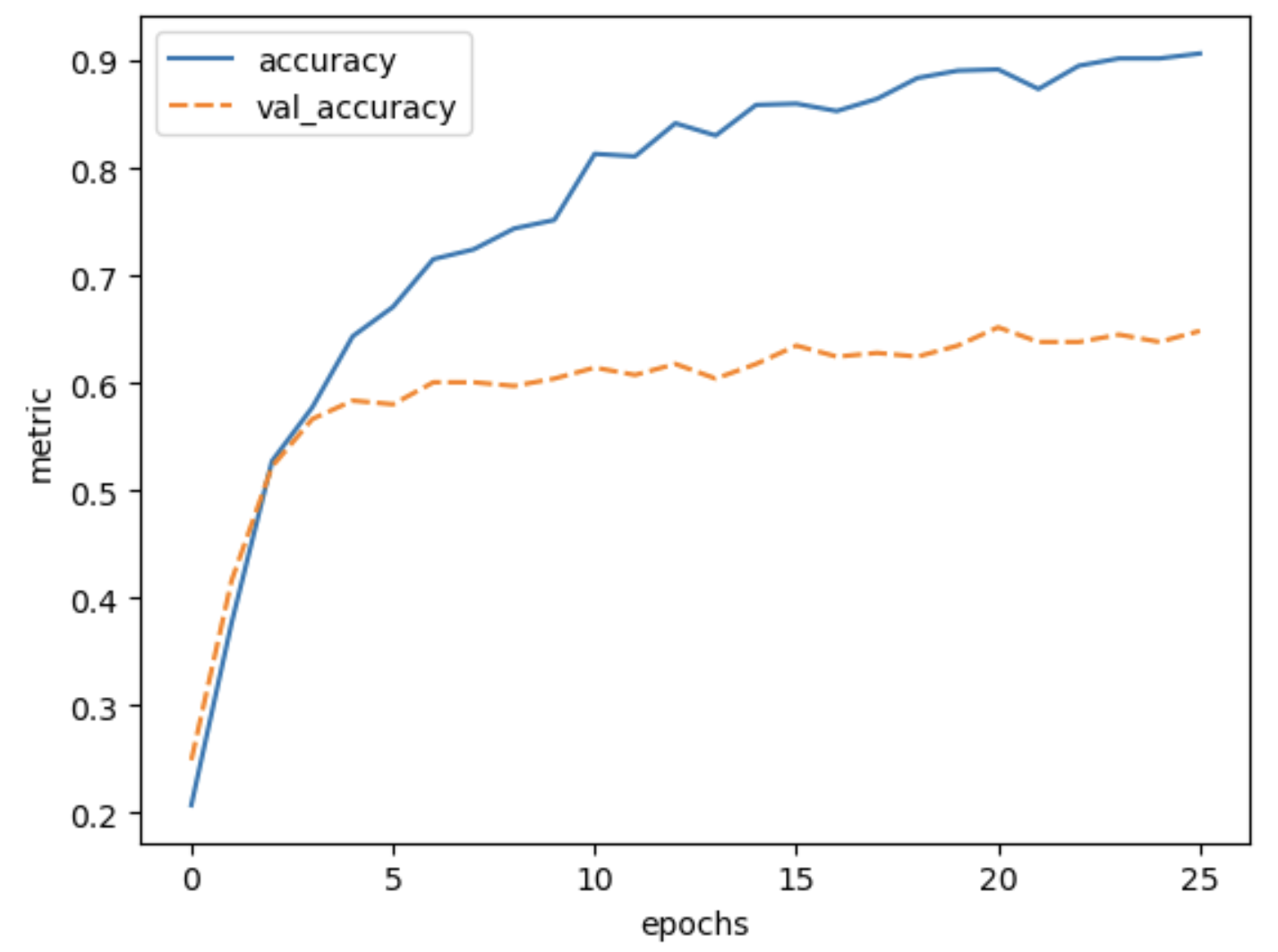 The final validation accuracy reaches 64%, this is a huge improvement
over 30% accuracy we reached with the simple convolutional neural
network that we build from scratch in the previous episode.
The final validation accuracy reaches 64%, this is a huge improvement
over 30% accuracy we reached with the simple convolutional neural
network that we build from scratch in the previous episode.
Fine-Tune the Top Layer of the Pretrained Model
So far, we’ve trained only the custom head while keeping the DenseNet121 base frozen. Let’s now unfreeze just the top layer group of the base model and observe how performance changes.
2. Recompile the model
Any time you change layer trainability, you must recompile the model.
Use the same optimizer and loss function as before: -
optimizer='adam' -
loss=SparseCategoricalCrossentropy(from_logits=True) -
metrics=['accuracy']
PYTHON
# 1. Unfreeze top block of base model
set_trainable = False
for layer in base_model.layers:
if 'conv5' in layer.name:
set_trainable = True
else:
set_trainable = False
layer.trainable = set_trainable
# 2. Recompile the model
model.compile(optimizer='adam',
              loss=keras.losses.SparseCategoricalCrossentropy(from_logits=True),
              metrics=['accuracy'])
# 3. Retrain the model
early_stopper = keras.callbacks.EarlyStopping(monitor='val_accuracy',
                              patience=5)
history_finetune = model.fit(train_images, train_labels,
batch_size=32,
epochs=30,
validation_data=(val_images, val_labels),
callbacks=[early_stopper])
# 4. Plot comparison
def plot_two_histories(h1, h2, label1='Frozen', label2='Finetuned'):
import pandas as pd
import matplotlib.pyplot as plt
df1 = pd.DataFrame(h1.history)
df2 = pd.DataFrame(h2.history)
plt.plot(df1['val_accuracy'], label=label1)
plt.plot(df2['val_accuracy'], label=label2)
plt.xlabel("Epochs")
plt.ylabel("Validation Accuracy")
plt.legend()
plt.title("Validation Accuracy: Frozen vs. Finetuned")
plt.show()
plot_two_histories(history, history_finetune)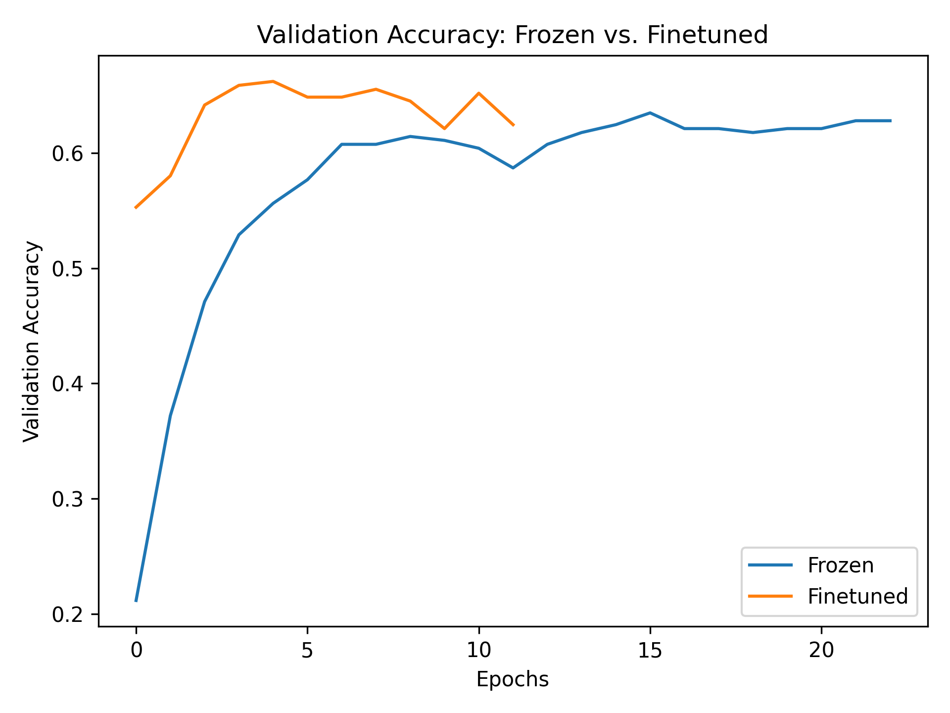
Discussion of results: Validation accuracy improved across all epochs compared to the frozen baseline. Training time also increased slightly, but the model was able to adapt better to the new dataset by fine-tuning the top convolutional block.
This makes sense: by unfreezing the last part of the base model, you’re allowing it to adjust high-level features to the new domain, while still keeping the earlier, general-purpose filters/feature-detectors of the model intact.
What happens if you unfreeze too many layers? If you unfreeze most or all of the base model:
- Training time increases significantly because more weights are being updated.
- The model may forget some of the general-purpose features it learned during pretraining. This is called “catastrophic forgetting.”
- Overfitting becomes more likely, especially if your dataset is small or noisy.
When does this approach work best?
Fine-tuning a few top layers is a good middle ground. You’re adapting the model without retraining everything from scratch. If your dataset is small or very different from the original ImageNet data, you should be careful not to unfreeze too many layers.
For most use cases: - Freeze most layers - Unfreeze the top block or two - Avoid full fine-tuning unless you have lots of data and compute
Concluding: The power of transfer learning
In many domains, large networks are available that have been trained on vast amounts of data, such as in computer vision and natural language processing. Using transfer learning, you can benefit from the knowledge that was captured from another machine learning task. In many fields, transfer learning will outperform models trained from scratch, especially if your dataset is small or of poor quality.
- Large pre-trained models capture generic knowledge about a domain
- Use the
keras.applicationsmodule to easily use pre-trained models for your own datasets