Ensemble methods

Overview

Questions

• What are ensemble methods, and why might they outperform a single model?
• How do stacking, bagging, and boosting differ conceptually and in practice?
• How can we use random forests in Scikit-Learn to improve on a single decision tree for classification?
• How can we combine different regression models into a single ensemble using VotingRegressor?

Objectives

• Define ensemble methods and explain why combining multiple models can reduce overfitting and improve robustness.
• Distinguish between stacking, bagging, and boosting and describe when each might be appropriate.
• Train and evaluate a RandomForestClassifier on the penguins dataset and compare its performance to a single decision tree.
• Inspect individual trees within a random forest and visualize decision boundaries to build intuition about how bagging works.
• Use Scikit-Learn’s VotingRegressor to stack multiple regression models (for example, random forest, gradient boosting, and linear regression) on the California housing dataset.
• Compare the performance of individual regressors to the stacked ensemble and interpret differences in test scores.
• Relate ensemble methods to bias–variance tradeoffs and overfitting, and discuss when ensembles are likely to be helpful in practice.

Ensemble methods

What’s better than one decision tree? Perhaps two? or three? How about enough trees to make up a forest? Ensemble methods bundle individual models together and use each of their outputs to contribute towards a final consensus for a given problem. Ensemble methods are based on the mantra that the whole is greater than the sum of the parts.

Thinking back to the classification episode with decision trees we quickly stumbled into the problem of overfitting our training data. If we combine predictions from a series of over/under fitting estimators then we can often produce a better final prediction than using a single reliable model - in the same way that humans often hear multiple opinions on a scenario before deciding a final outcome. Decision trees and regressions are often very sensitive to training outliers and so are well suited to be a part of an ensemble.

Ensemble methods are used for a variety of applciations including, but not limited to, search systems and object detection. We can use any model/estimator available in sci-kit learn to create an ensemble. There are three main methods to create ensembles approaches:

• Stacking
• Bagging
• Boosting

Let’s explore them in a bit more depth.

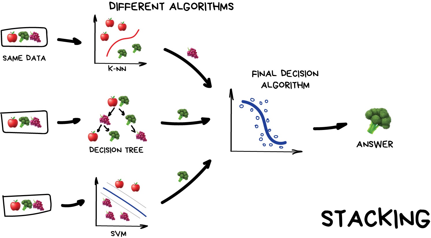
Stacking

This is where we train a series of different models/estimators on the same input data in parallel. We then take the output of each model and pass them into a final decision algorithm/model that makes the final prediction.

If we trained the same model multiple times on the same data we would expect very similar answers, and so the emphasis with stacking is to choose different models that can be used to build up a reliable concensus. Regression is then typically a good choice for the final decision-making model.

Stacking

Image from Vasily Zubarev via their blog

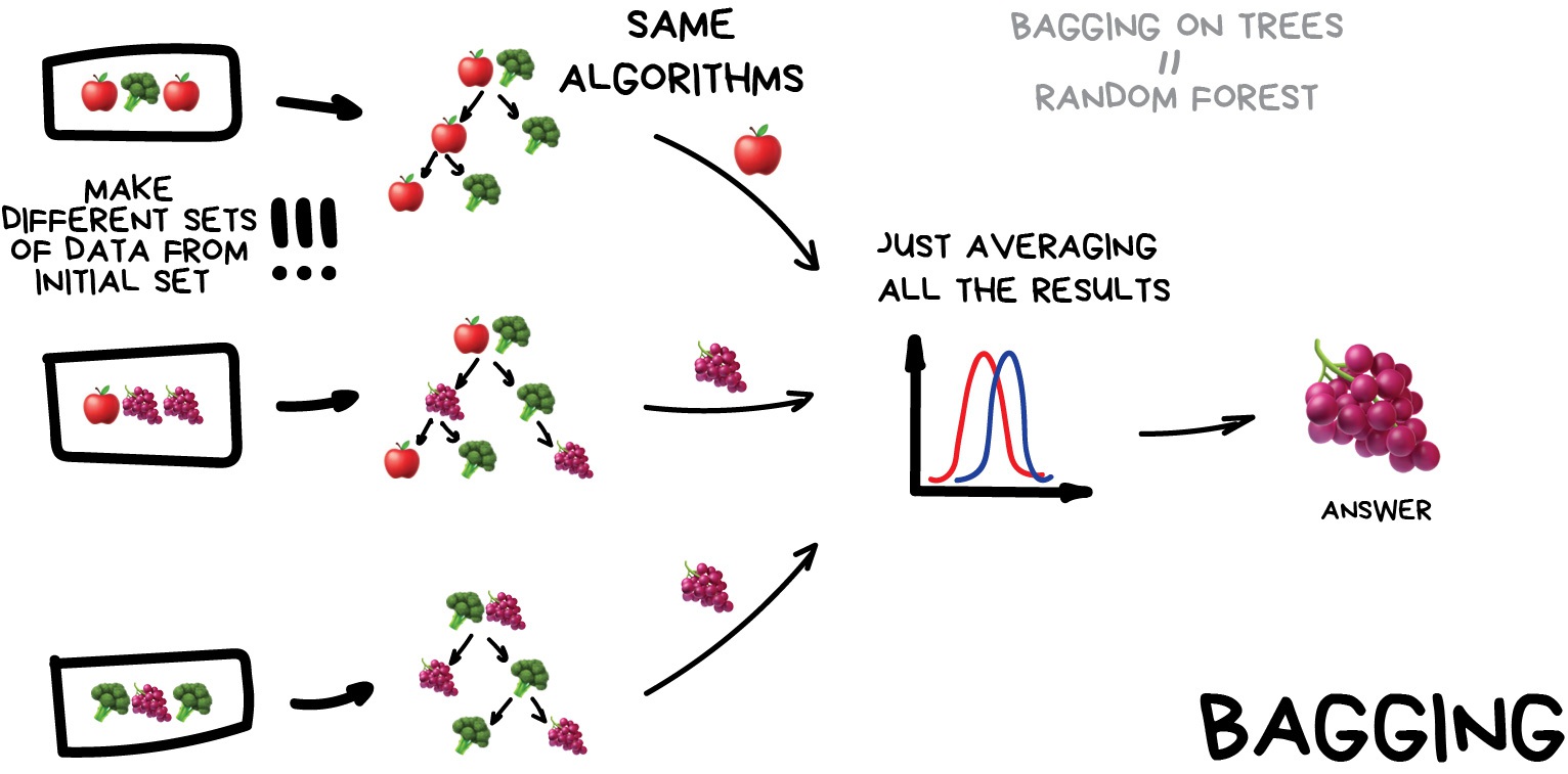
Bagging (a.k.a Bootstrap AGGregatING )

This is where we use the same model/estimator and fit it on different subsets of the training data. We can then average the results from each model to produce a final prediction. The subsets are random and may even repeat themselves.

How to remember: The name comes from combining two ideas, bootstrap (random sampling with replacement) and aggregating (combining predictions). Imagine putting your data into a “bag,” pulling out random samples (with replacement), training models on those samples, and combining their outputs.

The most common example is known as the Random Forest algorithm, which we’ll take a look at later on. Random Forests are typically used as a faster, computationally cheaper alternative to Neural Networks, which is ideal for real-time applications like camera face detection prompts.

Stacking

Image from Vasily Zubarev via their blog

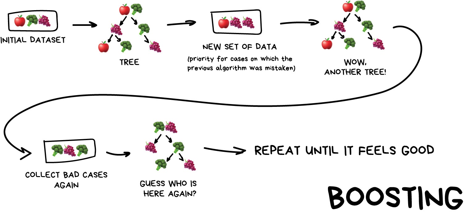
Boosting

This is where we train a single type of Model/estimator on an initial dataset, test it’s accuracy, and then subsequently train the same type of models on poorly predicted samples i.e. each new model pays most attention to data that were incorrectly predicted by the last one.

Just like for bagging, boosting is trained mostly on subsets, however in this case these subsets are not randomly generated but are instead built using poorly estimated predictions. Boosting can produce some very high accuracies by learning from it’s mistakes, but due to the iterative nature of these improvements it doesn’t parallelize well unlike the other ensemble methods. Despite this it can still be a faster, and computationally cheaper alternative to Neural Networks.

Stacking

Image from Vasily Zubarev via their blog

Ensemble summary

Machine learning jargon can often be hard to remember, so here is a quick summary of the 3 ensemble methods:

• Stacking - same dataset, different models, trained in parallel
• Bagging - different subsets, same models, trained in parallel
• Boosting - subsets of bad estimates, same models, trained in series

Which ensemble method is best?

Ensemble method	What it does	Best for	Avoid if
Stacking	Combines predictions from different models trained on the same dataset using a meta-model.	Leveraging diverse models to improve overall performance.	You need simple and fast models or lack diverse base learners.
Bagging	Trains the same model on different subsets of the data (via bootstrapping) and averages their results.	Reducing variance (e.g., overfitting) and stabilizing predictions in noisy/small datasets.	The problem requires reducing bias or the base model is already stable (e.g., linear regression).
Boosting	Sequentially trains models, focusing on correcting errors made by previous models.	Capturing complex patterns in large datasets and achieving the highest possible accuracy.	The dataset is small or noisy, or you lack computational resources.

Using Bagging (Random Forests) for a classification problem

In this session we’ll take another look at the penguins data and applying one of the most common bagging approaches, random forests, to try and solve our species classification problem. First we’ll load in the dataset and define a train and test split.

PYTHON

# import libraries
import numpy as np
import pandas as pd
import seaborn as sns
from sklearn.model_selection import train_test_split

# load penguins data
penguins = sns.load_dataset('penguins')

# prepare and define our data and targets
feature_names = ['bill_length_mm', 'bill_depth_mm', 'flipper_length_mm', 'body_mass_g']
penguins.dropna(subset=feature_names, inplace=True)

species_names = penguins['species'].unique()

X = penguins[feature_names]
y = penguins.species

# Split data in training and test set
X_train, X_test, y_train, y_test = train_test_split(X, y, test_size=0.2, random_state=5, stratify=y)

print("train size:", X_train.shape)
print("test size", X_test.shape)
X_train.head()

We’ll now take a look how we can use ensemble methods to perform a classification task such as identifying penguin species! We’re going to use a Random forest classifier available in scikit-learn which is a widely used example of a bagging approach.

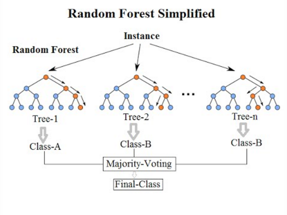
Random forests are built on decision trees and can provide another way to address over-fitting. Rather than classifying based on one single decision tree (which could overfit the data), an average of results of many trees can be derived for more robust/accurate estimates compared against single trees used in the ensemble.

Random Forests

Image from Venkatak Jagannath

We can now define a random forest estimator and train it using the penguin training data. We have a similar set of attritbutes to the DecisionTreeClassifier but with an extra parameter called n_estimators which is the number of trees in the forest.

PYTHON

from sklearn.ensemble import RandomForestClassifier
from sklearn.tree import plot_tree

# Define our model
# extra parameter called n_estimators which is number of trees in the forest
# a leaf is a class label at the end of the decision tree
forest = RandomForestClassifier(n_estimators=100, max_depth=5, min_samples_leaf=1, random_state=0) 

# train our model
forest.fit(X_train, y_train)

# Score our model
print(forest.score(X_test, y_test))

You might notice that we have a different value (hopefully increased) compared with the decision tree classifier used above on the same training data. Lets plot the first 5 trees in the forest to get an idea of how this model differs from a single decision tree.

PYTHON

import matplotlib.pyplot as plt

fig, axes = plt.subplots(nrows=1, ncols=5 ,figsize=(12,6))

# plot first 5 trees in forest
for index in range(0, 5):
    plot_tree(forest.estimators_[index], 
        class_names=species_names,
        feature_names=feature_names, 
        filled=True, 
        ax=axes[index])

    axes[index].set_title(f'Tree: {index}')
    
plt.show()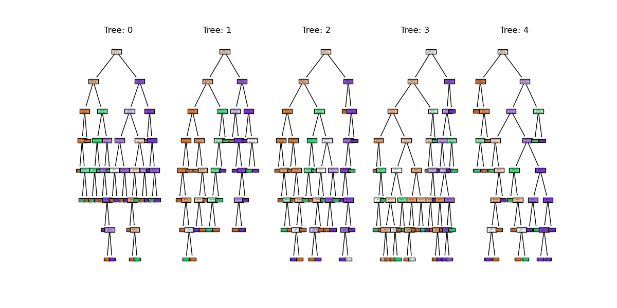

random forest trees

We can see the first 5 (of 100) trees that were fitted as part of the forest.

How votes are averaged in scikit-learn’s Random Forest

In scikit-learn, the RandomForestClassifier aggregates votes using averaged class probabilities rather than a strict majority vote.

• Each decision tree produces a probability distribution over classes for a given input (based on the proportion of samples from each class in the leaf node where that input ends up).
• The forest then takes the mean of those probabilities across all trees.
• The predicted class is the one with the highest average probability.

While traditional random forests are often described as using a “majority vote”, scikit-learn implements what’s called soft voting—averaging probabilities instead of labels.
This provides smoother decision boundaries and can improve calibration.

If we train the random forest estimator using the same two features from our decision tree example — what do we think the plot will look like?

PYTHON

# lets train a random forest for only two features (body mass and bill length)
from sklearn.inspection import DecisionBoundaryDisplay
f1 = feature_names[0]
f2 = feature_names[3]

# plot classification space for body mass and bill length with random forest
forest_2d = RandomForestClassifier(n_estimators=100, max_depth=5, min_samples_leaf=1, random_state=0)
forest_2d.fit(X_train[[f1, f2]], y_train)

# Lets plot the decision boundaries made by the model for the two trained features
d = DecisionBoundaryDisplay.from_estimator(forest_2d, X_train[[f1, f2]], grid_resolution=500))

sns.scatterplot(X_train, x=f1, y=f2, hue=y_train, palette="husl")
plt.show()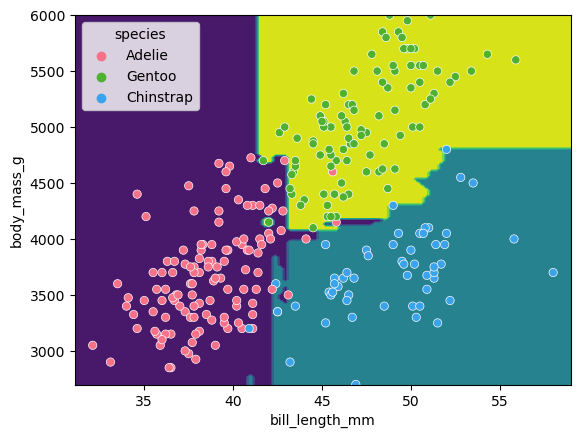

random forest clf space

There is still some overfitting indicated by the regions that contain only single points but using the same hyper-parameter settings used to fit the decision tree classifier, we can see that overfitting is reduced.

Stacking a regression problem

We’ve had a look at a bagging approach, but we’ll now take a look at a stacking approach and apply it to a regression problem. We’ll also introduce a new dataset to play around with.

California house price prediction

The California housing dataset for regression problems contains 8 training features such as, Median Income, House Age, Average Rooms, Average Bedrooms etc. for 20,640 properties. The target variable is the median house value for those 20,640 properties, note that all prices are in units of $100,000. This toy dataset is available as part of the scikit learn library. We’ll start by loading the dataset to very briefly inspect the attributes by printing them out.

PYTHON

import sklearn
from sklearn.datasets import fetch_california_housing

# load the dataset
X, y = fetch_california_housing(return_X_y=True, as_frame=True)

## All price variables are in units of $100,000
print(X.shape)
print(X.head())

print("Housing price as the target: ")

## Target is in units of $100,000
print(y.head())
print(y.shape)

For the the purposes of learning how to create and use ensemble methods and since it is a toy dataset, we will blindly use this dataset without inspecting it, cleaning or pre-processing it further.

Discussion

Exercise: Investigate and visualise the dataset

For this episode we simply want to learn how to build and use an Ensemble rather than actually solve a regression problem. To build up your skills as an ML practitioner, investigate and visualise this dataset. What can you say about the dataset itself, and what can you summarise about about any potential relationships or prediction problems?

Lets start by splitting the dataset into training and testing subsets:

PYTHON

# split into train and test sets, We are selecting an 80%-20% train-test split.
from sklearn.model_selection import train_test_split

X_train, X_test, y_train, y_test = train_test_split(X, y, test_size=0.2, random_state=5)

print(f'train size: {X_train.shape}')
print(f'test size: {X_test.shape}')

Lets stack a series of regression models. In the same way the RandomForest classifier derives a results from a series of trees, we will combine the results from a series of different models in our stack. This is done using what’s called an ensemble meta-estimator called a VotingRegressor.

We’ll apply a Voting regressor to a random forest, gradient boosting and linear regressor.

Callout

But wait, aren’t random forests/decision tree for classification problems?

Yes they are, but quite often in machine learning various models can be used to solve both regression and classification problems.

Decision trees in particular can be used to “predict” specific numerical values instead of categories, essentially by binning a group of values into a single value.

This works well for periodic/repeating numerical data. These trees are extremely sensitive to the data they are trained on, which makes them a very good model to use as a Random Forest.

Callout

But wait again, isn’t a random forest (and a gradient boosting model) an ensemble method instead of a regression model?

Yes they are, but they can be thought of as one big complex model used like any other model. The awesome thing about ensemble methods, and the generalisation of Scikit-Learn models, is that you can put an ensemble in an ensemble!

A VotingRegressor can train several base estimators on the whole dataset, and it can take the average of the individual predictions to form a final prediction.

PYTHON

from sklearn.ensemble import (
    GradientBoostingRegressor,
    RandomForestRegressor,
    VotingRegressor,
)
from sklearn.linear_model import LinearRegression

# Initialize estimators 
rf_reg = RandomForestRegressor(random_state=5)
gb_reg = GradientBoostingRegressor(random_state=5)
linear_reg = LinearRegression()
voting_reg = VotingRegressor([("rf", rf_reg), ("gb", gb_reg), ("lr", linear_reg)])

# fit/train voting estimator
voting_reg.fit(X_train, y_train)

# lets also fit/train the individual models for comparison
rf_reg.fit(X_train, y_train)
gb_reg.fit(X_train, y_train)
linear_reg.fit(X_train, y_train)

We fit the voting regressor in the same way we would fit a single model. When the voting regressor is instantiated we pass it a parameter containing a list of tuples that contain the estimators we wish to stack: in this case the random forest, gradient boosting and linear regressors. To get a sense of what this is doing lets predict the first 20 samples in the test portion of the data and plot the results.

PYTHON

import matplotlib.pyplot as plt

# make predictions
X_test_20 = X_test[:20] # first 20 for visualisation

rf_pred = rf_reg.predict(X_test_20)
gb_pred = gb_reg.predict(X_test_20)
linear_pred = linear_reg.predict(X_test_20)
voting_pred = voting_reg.predict(X_test_20)

plt.figure()
plt.plot(gb_pred,  "o", color="black", label="GradientBoostingRegressor")
plt.plot(rf_pred,  "o", color="blue", label="RandomForestRegressor")
plt.plot(linear_pred,  "o", color="green", label="LinearRegression")
plt.plot(voting_pred,  "x", color="red", ms=10, label="VotingRegressor")

plt.tick_params(axis="x", which="both", bottom=False, top=False, labelbottom=False)
plt.ylabel("predicted")
plt.xlabel("training samples")
plt.legend(loc="best")
plt.title("Regressor predictions and their average")

plt.show()

Regressor predictions and average from stack

Finally, lets see how the average compares against each single estimator in the stack?

PYTHON

print(f'random forest: {rf_reg.score(X_test, y_test)}')

print(f'gradient boost: {gb_reg.score(X_test, y_test)}')

print(f'linear regression: {linear_reg.score(X_test, y_test)}')

print(f'voting regressor: {voting_reg.score(X_test, y_test)}')

Each of our models score between 0.61-0.82, which at the high end is good, but at the low end is a pretty poor prediction accuracy score. Do note that the toy datasets are not representative of real world data. However what we can see is that the stacked result generated by the voting regressor fits different sub-models and then averages the individual predictions to form a final prediction. The benefit of this approach is that, it reduces overfitting and increases generalizability. Of course, we could try and improve our accuracy score by tweaking with our indivdual model hyperparameters, using more advaced boosted models or adjusting our training data features and train-test-split data.

Discussion

Exercise: Stacking a classification problem.

Scikit learn also has method for stacking ensemble classifiers sklearn.ensemble.VotingClassifier do you think you could apply a stack to the penguins dataset using a random forest, SVM and decision tree classifier, or a selection of any other classifier estimators available in sci-kit learn?

PYTHON

penguins = sns.load_dataset('penguins')

feature_names = ['bill_length_mm', 'bill_depth_mm', 'flipper_length_mm', 'body_mass_g']
penguins.dropna(subset=feature_names, inplace=True)

species_names = penguins['species'].unique()

# Define data and targets
X = penguins[feature_names]

y = penguins.species

# Split data in training and test set
from sklearn.model_selection import train_test_split

X_train, X_test, y_train, y_test = train_test_split(X, y, test_size=0.2, random_state=5)

print(f'train size: {X_train.shape}')
print(f'test size: {X_test.shape}')

The code above loads the penguins data and splits it into test and training portions. Have a play around with stacking some classifiers using the sklearn.ensemble.VotingClassifier using the code comments below as a guide.

PYTHON

# import classifiers 

# instantiate classifiers 

# fit classifiers

# instantiate voting classifier and fit data

# make predictions

# compare scores

Key Points

• Ensemble methods combine predictions from multiple models to produce more stable and accurate results than most single models.
• Bagging (such as random forests) trains the same model on different bootstrap samples and averages their predictions, usually reducing variance and overfitting.
• Boosting trains models in sequence, focusing later models on the mistakes of earlier ones, often improving accuracy at the cost of increased complexity and computation.
• Stacking uses a meta-model to combine the outputs of several diverse base models trained on the same data.
• Random forests often outperform single decision trees by averaging many shallow, noisy trees into a more robust classifier.
• VotingRegressor and VotingClassifier provide a simple way to stack multiple estimators in Scikit-Learn for regression or classification tasks.
• Choosing an ensemble method and tuning its hyperparameters is closely tied to the bias–variance tradeoff and the characteristics of the dataset.