Data Wrangling and Analyses with Tidyverse
Last updated on 2026-06-02 | Edit this page
Overview
Questions
- How can I manipulate data frames without repeating myself?
Objectives
- Explain the basic principle of tidy datasets
- Be able to load a tabular dataset using base R functions
- Describe what the
dplyrpackage in R is used for. - Apply common
dplyrfunctions to manipulate data in R. - Employ the ‘pipe’ operator to link together a sequence of functions.
- Employ the ‘mutate’ function to apply other chosen functions to existing columns and create new columns of data.
- Employ the ‘split-apply-combine’ concept to split the data into groups, apply analysis to each group, and combine the results.
Working with spreadsheets (tabular data)
A substantial amount of the data we work with in genomics will be tabular data, this is data arranged in rows and columns - also known as spreadsheets. We could write a whole lesson on how to work with spreadsheets effectively (actually we did). For our purposes, we want to remind you of a few principles before we work with our first set of example data:
1) Keep raw data separate from analyzed data
This is principle number one because if you can’t tell which files are the original raw data, you risk making some serious mistakes (e.g. drawing conclusion from data which have been manipulated in some unknown way).
2) Keep spreadsheet data Tidy
The simplest principle of Tidy data is that we have one row in our spreadsheet for each observation or sample, and one column for every variable that we measure or report on. As simple as this sounds, it’s very easily violated. Most data scientists agree that significant amounts of their time is spent tidying data for analysis. Read more about data organization in our lesson and in this paper.
3) Trust but verify
Finally, while you don’t need to be paranoid about data, you should have a plan for how you will prepare it for analysis. This a focus of this lesson. You probably already have a lot of intuition, expectations, assumptions about your data - the range of values you expect, how many values should have been recorded, etc. Of course, as the data get larger our human ability to keep track will start to fail (and yes, it can fail for small data sets too). R will help you to examine your data so that you can have greater confidence in your analysis, and its reproducibility.
Tip: Keep your raw data separate
When you work with data in R, you are not changing the original file
you loaded that data from. This is different than (for example) working
with a spreadsheet program where changing the value of the cell leaves
you one “save”-click away from overwriting the original file. You have
to purposely use a writing function (e.g. write.csv()) to
save data loaded into R. In that case, be sure to save the manipulated
data into a new file. More on this later in the lesson.
Base R (without additional packages) has a way of subsetting using brakets, which is handy, but it can be cumbersome and difficult to read, especially for complicated operations.
Luckily, the dplyr
package provides a number of very useful functions for manipulating data
frames (aka spreadsheets or tables of data) in a way that will reduce
repetition, reduce the probability of making errors, and probably even
save you some typing. As an added bonus, you might even find the
dplyr grammar easier to read.
Here we’re going to cover some of the most commonly used functions as
well as using pipes (%>%) to combine them:
glimpse()select()filter()group_by()summarize()mutate()-
inner_join(),full_join(),left_join(),right_join() - Extra -
pivot_longerandpivot_wider
Packages in R are sets of additional functions that let you do more
stuff in R. The functions we’ve been using, like str(),
come built into R; packages give you access to more functions. You need
to install a package and then load it to be able to use it.
R
install.packages("dplyr") ## installs dplyr package
install.packages("tidyr") ## installs tidyr package
install.packages("ggplot2") ## installs ggplot2 package
install.packages("readr") ## install readr package
Tip: Installing packages
It may be temping to install the tidyverse package, as
it contains many useful collection of packages for this lesson and
beyond. However, when teaching or following this lesson, we advise that
participants install dplyr, readr,
ggplot2, and tidyr individually as shown
above. Otherwise, a substaial amount of the lesson will be spend waiting
for the installation to complete.
You might get asked to choose a CRAN mirror – this is asking you to choose a site to download the package from. The choice doesn’t matter too much; I’d recommend choosing the RStudio mirror.
R
library("dplyr")          ## loads in dplyr package to use
library("tidyr")          ## loads in tidyr package to use
library("ggplot2")          ## loads in ggplot2 package to use
library("readr")          ## load in readr package to use
You only need to install a package once per computer, but you need to load it every time you open a new R session and want to use that package.
What is dplyr?
The package dplyr is a fairly new (2014) package that
tries to provide easy tools for the most common data manipulation tasks.
This package is also included in the tidyverse package,
which is a collection of eight different packages (dplyr,
ggplot2, tibble, tidyr,
readr, purrr, stringr, and
forcats). It is built to work directly with data frames.
The thinking behind it was largely inspired by the package
plyr which has been in use for some time but suffered from
being slow in some cases.dplyr addresses this by porting
much of the computation to C++. An additional feature is the ability to
work with data stored directly in an external database. The benefits of
doing this are that the data can be managed natively in a relational
database, queries can be conducted on that database, and only the
results of the query returned.
This addresses a common problem with R in that all operations are conducted in memory and thus the amount of data you can work with is limited by available memory. The database connections essentially remove that limitation in that you can have a database that is over 100s of GB, conduct queries on it directly and pull back just what you need for analysis in R.
Importing tabular data into R
There are several ways to import data into R. We will start loading
our data using the tidyverse package called readr and a
function called read_csv()
Exercise: Review the arguments of the
read_csv() function
Before using the read_csv() function, use R’s
help feature to answer the following questions.
Hint: Entering ‘?’ before the function name and then running
that line will bring up the help documentation. Also,
read_csv() is part of a family of functions for reading in
data called read_delim() so you will need to look for the
help page for read_delim() instead. When reading this
particular help be careful to pay attention to the ‘read_csv’ expression
under the ‘Usage’ heading. Other answers will be in the ‘Arguments’
heading.
What is the default parameter for ‘col_names’ in the
read_csv()function?What argument would you have to change to read a file that was delimited by semicolons (;) rather than commas?
What argument would you have to change to read skip commented lines (starting with #) at the beginning of a file (like our VCF file)? Hint: There are a couple of different possible answers to this question.
What argument would you have to change to read in only the first 10,000 rows of a very large file?
The
read_csv()function has the argument ‘col_names’ set to TRUE by default, this means the function always assumes the first row is header information, (i.e. column names)The
read_csv()function has the argument ‘delim’ which allows you to change the delimiter (aka separator) between columns. The function assumes commas are used as delimiters, as you would expect. Changing this parameter (e.g.delim=";") would now interpret semicolons as delimiters.To skip commented lines at the beginning of a file, there are a couple options. If the number of lines is consistent, we can use the
skipargument, for example,skip = 3will skip the first 3 lines of the file and then start reading in the header and data starting on line
- If the commented lines use a consistent delimeter (like #) we can
instead use the
commentargument, which skips any information after the charcter given. In this examplecomment = '#'will ignore lines starting with the hashtag/pound symbol. Note if you use both, skip will be executed first and then comment.
- You can set
n_maxto a numeric value (e.g.n_max=10000) to choose how many rows of a file you read in. This may be useful for very large files where not all the data is needed to test some data cleaning steps you are applying.
Hopefully, this exercise gets you thinking about using the provided help documentation in R. There are many arguments that exist, but which we wont have time to cover. Look here to get familiar with functions you use frequently, you may be surprised at what you find they can do.
Loading .csv files in tidy style
Now let’s load our vcf .csv file using read_csv():
OUTPUT
Rows: 801 Columns: 29
── Column specification ────────────────────────────────────────────────────────
Delimiter: ","
chr  (7): sample_id, CHROM, REF, ALT, DP4, Indiv, gt_GT_alleles
dbl (16): POS, QUAL, IDV, IMF, DP, VDB, RPB, MQB, BQB, MQSB, SGB, MQ0F, AC, ...
num  (1): gt_PL
lgl  (5): ID, FILTER, INDEL, ICB, HOB

ℹ Use `spec()` to retrieve the full column specification for this data.
ℹ Specify the column types or set `show_col_types = FALSE` to quiet this message.
Taking a quick look at data frames
Similar to str(), which comes built into R,
glimpse() is a dplyr function that (as the
name suggests) gives a glimpse of the data frame.
OUTPUT
Rows: 801
Columns: 29
$ sample_id     <chr> "SRR2584863", "SRR2584863", "SRR2584863", "SRR2584863", …
$ CHROM         <chr> "CP000819.1", "CP000819.1", "CP000819.1", "CP000819.1", …
$ POS           <dbl> 9972, 263235, 281923, 433359, 473901, 648692, 1331794, 1…
$ ID            <lgl> NA, NA, NA, NA, NA, NA, NA, NA, NA, NA, NA, NA, NA, NA, …
$ REF           <chr> "T", "G", "G", "CTTTTTTT", "CCGC", "C", "C", "G", "ACAGC…
$ ALT           <chr> "G", "T", "T", "CTTTTTTTT", "CCGCGC", "T", "A", "A", "AC…
$ QUAL          <dbl> 91.0000, 85.0000, 217.0000, 64.0000, 228.0000, 210.0000,…
$ FILTER        <lgl> NA, NA, NA, NA, NA, NA, NA, NA, NA, NA, NA, NA, NA, NA, …
$ INDEL         <lgl> FALSE, FALSE, FALSE, TRUE, TRUE, FALSE, FALSE, FALSE, TR…
$ IDV           <dbl> NA, NA, NA, 12, 9, NA, NA, NA, 2, 7, NA, NA, NA, NA, NA,…
$ IMF           <dbl> NA, NA, NA, 1.000000, 0.900000, NA, NA, NA, 0.666667, 1.…
$ DP            <dbl> 4, 6, 10, 12, 10, 10, 8, 11, 3, 7, 9, 20, 12, 19, 15, 10…
$ VDB           <dbl> 0.0257451, 0.0961330, 0.7740830, 0.4777040, 0.6595050, 0…
$ RPB           <dbl> NA, 1.000000, NA, NA, NA, NA, NA, NA, NA, NA, 0.900802, …
$ MQB           <dbl> NA, 1.0000000, NA, NA, NA, NA, NA, NA, NA, NA, 0.1501340…
$ BQB           <dbl> NA, 1.000000, NA, NA, NA, NA, NA, NA, NA, NA, 0.750668, …
$ MQSB          <dbl> NA, NA, 0.974597, 1.000000, 0.916482, 0.916482, 0.900802…
$ SGB           <dbl> -0.556411, -0.590765, -0.662043, -0.676189, -0.662043, -…
$ MQ0F          <dbl> 0.000000, 0.166667, 0.000000, 0.000000, 0.000000, 0.0000…
$ ICB           <lgl> NA, NA, NA, NA, NA, NA, NA, NA, NA, NA, NA, NA, NA, NA, …
$ HOB           <lgl> NA, NA, NA, NA, NA, NA, NA, NA, NA, NA, NA, NA, NA, NA, …
$ AC            <dbl> 1, 1, 1, 1, 1, 1, 1, 1, 1, 1, 1, 1, 1, 1, 1, 1, 1, 1, 1,…
$ AN            <dbl> 1, 1, 1, 1, 1, 1, 1, 1, 1, 1, 1, 1, 1, 1, 1, 1, 1, 1, 1,…
$ DP4           <chr> "0,0,0,4", "0,1,0,5", "0,0,4,5", "0,1,3,8", "1,0,2,7", "…
$ MQ            <dbl> 60, 33, 60, 60, 60, 60, 60, 60, 60, 60, 25, 60, 10, 60, …
$ Indiv         <chr> "/home/dcuser/dc_workshop/results/bam/SRR2584863.aligned…
$ gt_PL         <dbl> 1210, 1120, 2470, 910, 2550, 2400, 2080, 2550, 11128, 19…
$ gt_GT         <dbl> 1, 1, 1, 1, 1, 1, 1, 1, 1, 1, 1, 1, 1, 1, 1, 1, 1, 1, 1,…
$ gt_GT_alleles <chr> "G", "T", "T", "CTTTTTTTT", "CCGCGC", "T", "A", "A", "AC…
In the above output, we can already gather some information about
variants, such as the number of rows and columns, column
names, type of vector in the columns, and the first few entries of each
column. Although what we see is similar to outputs of
str(), this method gives a cleaner visual output.
Selecting columns and filtering rows
To select columns of a data frame, use select(). The
first argument to this function is the data frame
(variants), and the subsequent arguments are the columns to
keep.
R
select(variants, sample_id, REF, ALT, DP)
OUTPUT
# A tibble: 801 × 4
   sample_id  REF                              ALT                            DP
   <chr>      <chr>                            <chr>                       <dbl>
 1 SRR2584863 T                                G                               4
 2 SRR2584863 G                                T                               6
 3 SRR2584863 G                                T                              10
 4 SRR2584863 CTTTTTTT                         CTTTTTTTT                      12
 5 SRR2584863 CCGC                             CCGCGC                         10
 6 SRR2584863 C                                T                              10
 7 SRR2584863 C                                A                               8
 8 SRR2584863 G                                A                              11
 9 SRR2584863 ACAGCCAGCCAGCCAGCCAGCCAGCCAGCCAG ACAGCCAGCCAGCCAGCCAGCCAGCC…     3
10 SRR2584863 AT                               ATT                             7
# ℹ 791 more rows
To select all columns except certain ones, put a “-” in front of the variable to exclude it.
R
select(variants, -CHROM)
OUTPUT
# A tibble: 801 × 28
   sample_id      POS ID    REF      ALT    QUAL FILTER INDEL   IDV    IMF    DP
   <chr>        <dbl> <lgl> <chr>    <chr> <dbl> <lgl>  <lgl> <dbl>  <dbl> <dbl>
 1 SRR2584863    9972 NA    T        G        91 NA     FALSE    NA NA         4
 2 SRR2584863  263235 NA    G        T        85 NA     FALSE    NA NA         6
 3 SRR2584863  281923 NA    G        T       217 NA     FALSE    NA NA        10
 4 SRR2584863  433359 NA    CTTTTTTT CTTT…    64 NA     TRUE     12  1        12
 5 SRR2584863  473901 NA    CCGC     CCGC…   228 NA     TRUE      9  0.9      10
 6 SRR2584863  648692 NA    C        T       210 NA     FALSE    NA NA        10
 7 SRR2584863 1331794 NA    C        A       178 NA     FALSE    NA NA         8
 8 SRR2584863 1733343 NA    G        A       225 NA     FALSE    NA NA        11
 9 SRR2584863 2103887 NA    ACAGCCA… ACAG…    56 NA     TRUE      2  0.667     3
10 SRR2584863 2333538 NA    AT       ATT     167 NA     TRUE      7  1         7
# ℹ 791 more rows
# ℹ 17 more variables: VDB <dbl>, RPB <dbl>, MQB <dbl>, BQB <dbl>, MQSB <dbl>,
#   SGB <dbl>, MQ0F <dbl>, ICB <lgl>, HOB <lgl>, AC <dbl>, AN <dbl>, DP4 <chr>,
#   MQ <dbl>, Indiv <chr>, gt_PL <dbl>, gt_GT <dbl>, gt_GT_alleles <chr>
dplyr also provides useful functions to select columns
based on their names. For instance, ends_with() allows you
to select columns that ends with specific letters. For instance, if you
wanted to select columns that end with the letter “B”:
R
select(variants, ends_with("B"))
OUTPUT
# A tibble: 801 × 8
      VDB   RPB   MQB   BQB   MQSB    SGB ICB   HOB
    <dbl> <dbl> <dbl> <dbl>  <dbl>  <dbl> <lgl> <lgl>
 1 0.0257    NA    NA    NA NA     -0.556 NA    NA
 2 0.0961     1     1     1 NA     -0.591 NA    NA
 3 0.774     NA    NA    NA  0.975 -0.662 NA    NA
 4 0.478     NA    NA    NA  1     -0.676 NA    NA
 5 0.660     NA    NA    NA  0.916 -0.662 NA    NA
 6 0.268     NA    NA    NA  0.916 -0.670 NA    NA
 7 0.624     NA    NA    NA  0.901 -0.651 NA    NA
 8 0.992     NA    NA    NA  1.01  -0.670 NA    NA
 9 0.902     NA    NA    NA  1     -0.454 NA    NA
10 0.568     NA    NA    NA  1.01  -0.617 NA    NA
# ℹ 791 more rows
Challenge
Create a table that contains all the columns with the letter “i” and
column “POS”, without columns “Indiv” and “FILTER”. Hint: look at for a
function called contains(), which can be found in the help
documentation for ends with we just covered (?ends_with).
Note that contains() is not case sensistive.
R
# First, we select "POS" and all columns with letter "i". This will contain columns Indiv and FILTER.
variants_subset <- select(variants, POS, contains("i"))
# Next, we remove columns Indiv and FILTER
variants_result <- select(variants_subset, -Indiv, -FILTER)
variants_result
OUTPUT
# A tibble: 801 × 7
       POS sample_id  ID    INDEL   IDV    IMF ICB
     <dbl> <chr>      <lgl> <lgl> <dbl>  <dbl> <lgl>
 1    9972 SRR2584863 NA    FALSE    NA NA     NA
 2  263235 SRR2584863 NA    FALSE    NA NA     NA
 3  281923 SRR2584863 NA    FALSE    NA NA     NA
 4  433359 SRR2584863 NA    TRUE     12  1     NA
 5  473901 SRR2584863 NA    TRUE      9  0.9   NA
 6  648692 SRR2584863 NA    FALSE    NA NA     NA
 7 1331794 SRR2584863 NA    FALSE    NA NA     NA
 8 1733343 SRR2584863 NA    FALSE    NA NA     NA
 9 2103887 SRR2584863 NA    TRUE      2  0.667 NA
10 2333538 SRR2584863 NA    TRUE      7  1     NA
# ℹ 791 more rows
Challenge (continued)
We can also get to variants_result in one line of
code:
R
variants_result <- select(variants, POS, contains("i"), -Indiv, -FILTER)
variants_result
OUTPUT
# A tibble: 801 × 7
       POS sample_id  ID    INDEL   IDV    IMF ICB
     <dbl> <chr>      <lgl> <lgl> <dbl>  <dbl> <lgl>
 1    9972 SRR2584863 NA    FALSE    NA NA     NA
 2  263235 SRR2584863 NA    FALSE    NA NA     NA
 3  281923 SRR2584863 NA    FALSE    NA NA     NA
 4  433359 SRR2584863 NA    TRUE     12  1     NA
 5  473901 SRR2584863 NA    TRUE      9  0.9   NA
 6  648692 SRR2584863 NA    FALSE    NA NA     NA
 7 1331794 SRR2584863 NA    FALSE    NA NA     NA
 8 1733343 SRR2584863 NA    FALSE    NA NA     NA
 9 2103887 SRR2584863 NA    TRUE      2  0.667 NA
10 2333538 SRR2584863 NA    TRUE      7  1     NA
# ℹ 791 more rows
To choose rows, use filter():
R
filter(variants, sample_id == "SRR2584863")
OUTPUT
# A tibble: 25 × 29
   sample_id  CHROM        POS ID    REF   ALT    QUAL FILTER INDEL   IDV    IMF
   <chr>      <chr>      <dbl> <lgl> <chr> <chr> <dbl> <lgl>  <lgl> <dbl>  <dbl>
 1 SRR2584863 CP000819… 9.97e3 NA    T     G        91 NA     FALSE    NA NA
 2 SRR2584863 CP000819… 2.63e5 NA    G     T        85 NA     FALSE    NA NA
 3 SRR2584863 CP000819… 2.82e5 NA    G     T       217 NA     FALSE    NA NA
 4 SRR2584863 CP000819… 4.33e5 NA    CTTT… CTTT…    64 NA     TRUE     12  1
 5 SRR2584863 CP000819… 4.74e5 NA    CCGC  CCGC…   228 NA     TRUE      9  0.9
 6 SRR2584863 CP000819… 6.49e5 NA    C     T       210 NA     FALSE    NA NA
 7 SRR2584863 CP000819… 1.33e6 NA    C     A       178 NA     FALSE    NA NA
 8 SRR2584863 CP000819… 1.73e6 NA    G     A       225 NA     FALSE    NA NA
 9 SRR2584863 CP000819… 2.10e6 NA    ACAG… ACAG…    56 NA     TRUE      2  0.667
10 SRR2584863 CP000819… 2.33e6 NA    AT    ATT     167 NA     TRUE      7  1
# ℹ 15 more rows
# ℹ 18 more variables: DP <dbl>, VDB <dbl>, RPB <dbl>, MQB <dbl>, BQB <dbl>,
#   MQSB <dbl>, SGB <dbl>, MQ0F <dbl>, ICB <lgl>, HOB <lgl>, AC <dbl>,
#   AN <dbl>, DP4 <chr>, MQ <dbl>, Indiv <chr>, gt_PL <dbl>, gt_GT <dbl>,
#   gt_GT_alleles <chr>
filter() will keep all the rows that match the
conditions that are provided. Here are a few examples:
R
# rows for which the reference genome has T or G
filter(variants, REF %in% c("T", "G"))
OUTPUT
# A tibble: 340 × 29
   sample_id CHROM    POS ID    REF   ALT    QUAL FILTER INDEL   IDV   IMF    DP
   <chr>     <chr>  <dbl> <lgl> <chr> <chr> <dbl> <lgl>  <lgl> <dbl> <dbl> <dbl>
 1 SRR25848… CP00… 9.97e3 NA    T     G      91   NA     FALSE    NA    NA     4
 2 SRR25848… CP00… 2.63e5 NA    G     T      85   NA     FALSE    NA    NA     6
 3 SRR25848… CP00… 2.82e5 NA    G     T     217   NA     FALSE    NA    NA    10
 4 SRR25848… CP00… 1.73e6 NA    G     A     225   NA     FALSE    NA    NA    11
 5 SRR25848… CP00… 2.62e6 NA    G     T      31.9 NA     FALSE    NA    NA    12
 6 SRR25848… CP00… 3.00e6 NA    G     A     225   NA     FALSE    NA    NA    15
 7 SRR25848… CP00… 3.91e6 NA    G     T     225   NA     FALSE    NA    NA    10
 8 SRR25848… CP00… 9.97e3 NA    T     G     214   NA     FALSE    NA    NA    10
 9 SRR25848… CP00… 1.06e4 NA    G     A     225   NA     FALSE    NA    NA    11
10 SRR25848… CP00… 6.40e4 NA    G     A     225   NA     FALSE    NA    NA    18
# ℹ 330 more rows
# ℹ 17 more variables: VDB <dbl>, RPB <dbl>, MQB <dbl>, BQB <dbl>, MQSB <dbl>,
#   SGB <dbl>, MQ0F <dbl>, ICB <lgl>, HOB <lgl>, AC <dbl>, AN <dbl>, DP4 <chr>,
#   MQ <dbl>, Indiv <chr>, gt_PL <dbl>, gt_GT <dbl>, gt_GT_alleles <chr>
R
# rows that have TRUE in the column INDEL
filter(variants, INDEL)
OUTPUT
# A tibble: 101 × 29
   sample_id CHROM    POS ID    REF   ALT    QUAL FILTER INDEL   IDV   IMF    DP
   <chr>     <chr>  <dbl> <lgl> <chr> <chr> <dbl> <lgl>  <lgl> <dbl> <dbl> <dbl>
 1 SRR25848… CP00… 4.33e5 NA    CTTT… CTTT…  64   NA     TRUE     12 1        12
 2 SRR25848… CP00… 4.74e5 NA    CCGC  CCGC… 228   NA     TRUE      9 0.9      10
 3 SRR25848… CP00… 2.10e6 NA    ACAG… ACAG…  56   NA     TRUE      2 0.667     3
 4 SRR25848… CP00… 2.33e6 NA    AT    ATT   167   NA     TRUE      7 1         7
 5 SRR25848… CP00… 3.90e6 NA    A     AC     43.4 NA     TRUE      2 1         2
 6 SRR25848… CP00… 4.43e6 NA    TGG   T     228   NA     TRUE     10 1        10
 7 SRR25848… CP00… 1.48e5 NA    AGGGG AGGG… 122   NA     TRUE      8 1         8
 8 SRR25848… CP00… 1.58e5 NA    GTTT… GTTT…  19.5 NA     TRUE      6 1         6
 9 SRR25848… CP00… 1.73e5 NA    CAA   CA    180   NA     TRUE     11 1        11
10 SRR25848… CP00… 1.75e5 NA    GAA   GA    194   NA     TRUE     10 1        10
# ℹ 91 more rows
# ℹ 17 more variables: VDB <dbl>, RPB <dbl>, MQB <dbl>, BQB <dbl>, MQSB <dbl>,
#   SGB <dbl>, MQ0F <dbl>, ICB <lgl>, HOB <lgl>, AC <dbl>, AN <dbl>, DP4 <chr>,
#   MQ <dbl>, Indiv <chr>, gt_PL <dbl>, gt_GT <dbl>, gt_GT_alleles <chr>
R
# rows that don't have missing data in the IDV column
filter(variants, !is.na(IDV))
OUTPUT
# A tibble: 101 × 29
   sample_id CHROM    POS ID    REF   ALT    QUAL FILTER INDEL   IDV   IMF    DP
   <chr>     <chr>  <dbl> <lgl> <chr> <chr> <dbl> <lgl>  <lgl> <dbl> <dbl> <dbl>
 1 SRR25848… CP00… 4.33e5 NA    CTTT… CTTT…  64   NA     TRUE     12 1        12
 2 SRR25848… CP00… 4.74e5 NA    CCGC  CCGC… 228   NA     TRUE      9 0.9      10
 3 SRR25848… CP00… 2.10e6 NA    ACAG… ACAG…  56   NA     TRUE      2 0.667     3
 4 SRR25848… CP00… 2.33e6 NA    AT    ATT   167   NA     TRUE      7 1         7
 5 SRR25848… CP00… 3.90e6 NA    A     AC     43.4 NA     TRUE      2 1         2
 6 SRR25848… CP00… 4.43e6 NA    TGG   T     228   NA     TRUE     10 1        10
 7 SRR25848… CP00… 1.48e5 NA    AGGGG AGGG… 122   NA     TRUE      8 1         8
 8 SRR25848… CP00… 1.58e5 NA    GTTT… GTTT…  19.5 NA     TRUE      6 1         6
 9 SRR25848… CP00… 1.73e5 NA    CAA   CA    180   NA     TRUE     11 1        11
10 SRR25848… CP00… 1.75e5 NA    GAA   GA    194   NA     TRUE     10 1        10
# ℹ 91 more rows
# ℹ 17 more variables: VDB <dbl>, RPB <dbl>, MQB <dbl>, BQB <dbl>, MQSB <dbl>,
#   SGB <dbl>, MQ0F <dbl>, ICB <lgl>, HOB <lgl>, AC <dbl>, AN <dbl>, DP4 <chr>,
#   MQ <dbl>, Indiv <chr>, gt_PL <dbl>, gt_GT <dbl>, gt_GT_alleles <chr>
We have a column titled “QUAL”. This is a Phred-scaled confidence
score that a polymorphism exists at this position given the sequencing
data. Lower QUAL scores indicate low probability of a polymorphism
existing at that site. filter() can be useful for selecting
mutations that have a QUAL score above a certain threshold:
R
# rows with QUAL values greater than or equal to 100
filter(variants, QUAL >= 100)
OUTPUT
# A tibble: 666 × 29
   sample_id CHROM    POS ID    REF   ALT    QUAL FILTER INDEL   IDV   IMF    DP
   <chr>     <chr>  <dbl> <lgl> <chr> <chr> <dbl> <lgl>  <lgl> <dbl> <dbl> <dbl>
 1 SRR25848… CP00… 2.82e5 NA    G     T       217 NA     FALSE    NA  NA      10
 2 SRR25848… CP00… 4.74e5 NA    CCGC  CCGC…   228 NA     TRUE      9   0.9    10
 3 SRR25848… CP00… 6.49e5 NA    C     T       210 NA     FALSE    NA  NA      10
 4 SRR25848… CP00… 1.33e6 NA    C     A       178 NA     FALSE    NA  NA       8
 5 SRR25848… CP00… 1.73e6 NA    G     A       225 NA     FALSE    NA  NA      11
 6 SRR25848… CP00… 2.33e6 NA    AT    ATT     167 NA     TRUE      7   1       7
 7 SRR25848… CP00… 2.41e6 NA    A     C       104 NA     FALSE    NA  NA       9
 8 SRR25848… CP00… 2.45e6 NA    A     C       225 NA     FALSE    NA  NA      20
 9 SRR25848… CP00… 2.67e6 NA    A     T       225 NA     FALSE    NA  NA      19
10 SRR25848… CP00… 3.00e6 NA    G     A       225 NA     FALSE    NA  NA      15
# ℹ 656 more rows
# ℹ 17 more variables: VDB <dbl>, RPB <dbl>, MQB <dbl>, BQB <dbl>, MQSB <dbl>,
#   SGB <dbl>, MQ0F <dbl>, ICB <lgl>, HOB <lgl>, AC <dbl>, AN <dbl>, DP4 <chr>,
#   MQ <dbl>, Indiv <chr>, gt_PL <dbl>, gt_GT <dbl>, gt_GT_alleles <chr>
filter() allows you to combine multiple conditions. You
can separate them using a , as arguments to the function,
they will be combined using the & (AND) logical
operator. If you need to use the | (OR) logical operator,
you can specify it explicitly:
R
# this is equivalent to:
#   filter(variants, sample_id == "SRR2584863" & QUAL >= 100)
filter(variants, sample_id == "SRR2584863", QUAL >= 100)
OUTPUT
# A tibble: 19 × 29
   sample_id CHROM    POS ID    REF   ALT    QUAL FILTER INDEL   IDV   IMF    DP
   <chr>     <chr>  <dbl> <lgl> <chr> <chr> <dbl> <lgl>  <lgl> <dbl> <dbl> <dbl>
 1 SRR25848… CP00… 2.82e5 NA    G     T       217 NA     FALSE    NA  NA      10
 2 SRR25848… CP00… 4.74e5 NA    CCGC  CCGC…   228 NA     TRUE      9   0.9    10
 3 SRR25848… CP00… 6.49e5 NA    C     T       210 NA     FALSE    NA  NA      10
 4 SRR25848… CP00… 1.33e6 NA    C     A       178 NA     FALSE    NA  NA       8
 5 SRR25848… CP00… 1.73e6 NA    G     A       225 NA     FALSE    NA  NA      11
 6 SRR25848… CP00… 2.33e6 NA    AT    ATT     167 NA     TRUE      7   1       7
 7 SRR25848… CP00… 2.41e6 NA    A     C       104 NA     FALSE    NA  NA       9
 8 SRR25848… CP00… 2.45e6 NA    A     C       225 NA     FALSE    NA  NA      20
 9 SRR25848… CP00… 2.67e6 NA    A     T       225 NA     FALSE    NA  NA      19
10 SRR25848… CP00… 3.00e6 NA    G     A       225 NA     FALSE    NA  NA      15
11 SRR25848… CP00… 3.34e6 NA    A     C       211 NA     FALSE    NA  NA      10
12 SRR25848… CP00… 3.40e6 NA    C     A       225 NA     FALSE    NA  NA      14
13 SRR25848… CP00… 3.48e6 NA    A     G       200 NA     FALSE    NA  NA       9
14 SRR25848… CP00… 3.49e6 NA    A     C       225 NA     FALSE    NA  NA      13
15 SRR25848… CP00… 3.91e6 NA    G     T       225 NA     FALSE    NA  NA      10
16 SRR25848… CP00… 4.10e6 NA    A     G       225 NA     FALSE    NA  NA      16
17 SRR25848… CP00… 4.20e6 NA    A     C       225 NA     FALSE    NA  NA      11
18 SRR25848… CP00… 4.43e6 NA    TGG   T       228 NA     TRUE     10   1      10
19 SRR25848… CP00… 4.62e6 NA    A     C       185 NA     FALSE    NA  NA       9
# ℹ 17 more variables: VDB <dbl>, RPB <dbl>, MQB <dbl>, BQB <dbl>, MQSB <dbl>,
#   SGB <dbl>, MQ0F <dbl>, ICB <lgl>, HOB <lgl>, AC <dbl>, AN <dbl>, DP4 <chr>,
#   MQ <dbl>, Indiv <chr>, gt_PL <dbl>, gt_GT <dbl>, gt_GT_alleles <chr>
R
# using `|` logical operator
filter(variants, sample_id == "SRR2584863", (MQ >= 50 | QUAL >= 100))
OUTPUT
# A tibble: 23 × 29
   sample_id  CHROM        POS ID    REF   ALT    QUAL FILTER INDEL   IDV    IMF
   <chr>      <chr>      <dbl> <lgl> <chr> <chr> <dbl> <lgl>  <lgl> <dbl>  <dbl>
 1 SRR2584863 CP000819… 9.97e3 NA    T     G        91 NA     FALSE    NA NA
 2 SRR2584863 CP000819… 2.82e5 NA    G     T       217 NA     FALSE    NA NA
 3 SRR2584863 CP000819… 4.33e5 NA    CTTT… CTTT…    64 NA     TRUE     12  1
 4 SRR2584863 CP000819… 4.74e5 NA    CCGC  CCGC…   228 NA     TRUE      9  0.9
 5 SRR2584863 CP000819… 6.49e5 NA    C     T       210 NA     FALSE    NA NA
 6 SRR2584863 CP000819… 1.33e6 NA    C     A       178 NA     FALSE    NA NA
 7 SRR2584863 CP000819… 1.73e6 NA    G     A       225 NA     FALSE    NA NA
 8 SRR2584863 CP000819… 2.10e6 NA    ACAG… ACAG…    56 NA     TRUE      2  0.667
 9 SRR2584863 CP000819… 2.33e6 NA    AT    ATT     167 NA     TRUE      7  1
10 SRR2584863 CP000819… 2.41e6 NA    A     C       104 NA     FALSE    NA NA
# ℹ 13 more rows
# ℹ 18 more variables: DP <dbl>, VDB <dbl>, RPB <dbl>, MQB <dbl>, BQB <dbl>,
#   MQSB <dbl>, SGB <dbl>, MQ0F <dbl>, ICB <lgl>, HOB <lgl>, AC <dbl>,
#   AN <dbl>, DP4 <chr>, MQ <dbl>, Indiv <chr>, gt_PL <dbl>, gt_GT <dbl>,
#   gt_GT_alleles <chr>
Challenge
Select all the mutations that occurred between the positions 1e6 (one million) and 2e6 (inclusive) that have a QUAL greater than 200, and exclude INDEL mutations. Hint: to flip logical values such as TRUE to a FALSE, we can use to negation symbol “!”. (eg. !TRUE == FALSE).
R
filter(variants, POS >= 1e6 & POS <= 2e6, QUAL > 200, !INDEL)
OUTPUT
# A tibble: 77 × 29
   sample_id CHROM    POS ID    REF   ALT    QUAL FILTER INDEL   IDV   IMF    DP
   <chr>     <chr>  <dbl> <lgl> <chr> <chr> <dbl> <lgl>  <lgl> <dbl> <dbl> <dbl>
 1 SRR25848… CP00… 1.73e6 NA    G     A       225 NA     FALSE    NA    NA    11
 2 SRR25848… CP00… 1.00e6 NA    A     G       225 NA     FALSE    NA    NA    15
 3 SRR25848… CP00… 1.02e6 NA    A     G       225 NA     FALSE    NA    NA    12
 4 SRR25848… CP00… 1.06e6 NA    C     T       225 NA     FALSE    NA    NA    17
 5 SRR25848… CP00… 1.06e6 NA    A     G       206 NA     FALSE    NA    NA     9
 6 SRR25848… CP00… 1.07e6 NA    G     T       225 NA     FALSE    NA    NA    11
 7 SRR25848… CP00… 1.07e6 NA    T     C       225 NA     FALSE    NA    NA    12
 8 SRR25848… CP00… 1.10e6 NA    C     T       225 NA     FALSE    NA    NA    15
 9 SRR25848… CP00… 1.11e6 NA    C     T       212 NA     FALSE    NA    NA     9
10 SRR25848… CP00… 1.11e6 NA    A     G       225 NA     FALSE    NA    NA    14
# ℹ 67 more rows
# ℹ 17 more variables: VDB <dbl>, RPB <dbl>, MQB <dbl>, BQB <dbl>, MQSB <dbl>,
#   SGB <dbl>, MQ0F <dbl>, ICB <lgl>, HOB <lgl>, AC <dbl>, AN <dbl>, DP4 <chr>,
#   MQ <dbl>, Indiv <chr>, gt_PL <dbl>, gt_GT <dbl>, gt_GT_alleles <chr>
Pipes
But what if you wanted to select and filter? We can do this with
pipes. Pipes let you take the output of one function and send it
directly to the next, which is useful when you need to many things to
the same data set. It was possible to do this before pipes were added to
R, but it was much messier and more difficult. Pipes in R look like
%>% and are made available via the magrittr
package, which is installed as part of dplyr. If you use
RStudio, you can type the pipe with Ctrl + Shift +
M if you’re using a PC, or Cmd + Shift
+ M if you’re using a Mac.
R
variants %>%
  filter(sample_id == "SRR2584863") %>%
  select(REF, ALT, DP)
OUTPUT
# A tibble: 25 × 3
   REF                              ALT                                       DP
   <chr>                            <chr>                                  <dbl>
 1 T                                G                                          4
 2 G                                T                                          6
 3 G                                T                                         10
 4 CTTTTTTT                         CTTTTTTTT                                 12
 5 CCGC                             CCGCGC                                    10
 6 C                                T                                         10
 7 C                                A                                          8
 8 G                                A                                         11
 9 ACAGCCAGCCAGCCAGCCAGCCAGCCAGCCAG ACAGCCAGCCAGCCAGCCAGCCAGCCAGCCAGCCAGC…     3
10 AT                               ATT                                        7
# ℹ 15 more rows
In the above code, we use the pipe to send the variants
data set first through filter(), to keep rows where
sample_id matches a particular sample, and then through
select() to keep only the REF,
ALT, and DP columns. Since %>%
takes the object on its left and passes it as the first argument to the
function on its right, we don’t need to explicitly include the data
frame as an argument to the filter() and
select() functions any more.
Same code with no pipes
Without pipes the code would look like the following.
R
select(filter(variants, sample_id == "SRR2584863"), REF, ALT, DP)
OUTPUT
# A tibble: 25 × 3
   REF                              ALT                                       DP
   <chr>                            <chr>                                  <dbl>
 1 T                                G                                          4
 2 G                                T                                          6
 3 G                                T                                         10
 4 CTTTTTTT                         CTTTTTTTT                                 12
 5 CCGC                             CCGCGC                                    10
 6 C                                T                                         10
 7 C                                A                                          8
 8 G                                A                                         11
 9 ACAGCCAGCCAGCCAGCCAGCCAGCCAGCCAG ACAGCCAGCCAGCCAGCCAGCCAGCCAGCCAGCCAGC…     3
10 AT                               ATT                                        7
# ℹ 15 more rows
In this code we do the filter first and then wrap the
select function around it to use the output of the
filter command as the input fo the select
function. While both are valid, using pipes is considered more readable
as it displays the functions in top down order, instead of inside out
order.
Some may find it helpful to read the pipe like the word “then”. For
instance, in the above example, we took the data frame
variants, then we filtered for rows
where sample_id was SRR2584863, then we
selected the REF, ALT, and
DP columns. The dplyr
functions by themselves are somewhat simple, but by combining them into
linear workflows with the pipe, we can accomplish more complex
manipulations of data frames.
If we want to create a new object with this smaller version of the data we can do so by assigning it a new name:
R
SRR2584863_variants <- variants %>%
  filter(sample_id == "SRR2584863") %>%
  select(REF, ALT, DP)
This new object includes all of the data from this sample. Let’s look at just the first six rows to confirm it’s what we want:
R
SRR2584863_variants
OUTPUT
# A tibble: 25 × 3
   REF                              ALT                                       DP
   <chr>                            <chr>                                  <dbl>
 1 T                                G                                          4
 2 G                                T                                          6
 3 G                                T                                         10
 4 CTTTTTTT                         CTTTTTTTT                                 12
 5 CCGC                             CCGCGC                                    10
 6 C                                T                                         10
 7 C                                A                                          8
 8 G                                A                                         11
 9 ACAGCCAGCCAGCCAGCCAGCCAGCCAGCCAG ACAGCCAGCCAGCCAGCCAGCCAGCCAGCCAGCCAGC…     3
10 AT                               ATT                                        7
# ℹ 15 more rows
We can use the head() and tail() functions
to look at the first or last six rows. There is also a more versitle
tidyverse function slice(), that allows users to specify a
range to view:
R
SRR2584863_variants %>% head()
OUTPUT
# A tibble: 6 × 3
  REF      ALT          DP
  <chr>    <chr>     <dbl>
1 T        G             4
2 G        T             6
3 G        T            10
4 CTTTTTTT CTTTTTTTT    12
5 CCGC     CCGCGC       10
6 C        T            10
R
SRR2584863_variants %>% tail()
OUTPUT
# A tibble: 6 × 3
  REF   ALT      DP
  <chr> <chr> <dbl>
1 A     AC        2
2 G     T        10
3 A     G        16
4 A     C        11
5 TGG   T        10
6 A     C         9
R
SRR2584863_variants %>% slice(4:10) # shows rows 4-10 instead
OUTPUT
# A tibble: 7 × 3
  REF                              ALT                                        DP
  <chr>                            <chr>                                   <dbl>
1 CTTTTTTT                         CTTTTTTTT                                  12
2 CCGC                             CCGCGC                                     10
3 C                                T                                          10
4 C                                A                                           8
5 G                                A                                          11
6 ACAGCCAGCCAGCCAGCCAGCCAGCCAGCCAG ACAGCCAGCCAGCCAGCCAGCCAGCCAGCCAGCCAGCC…     3
7 AT ATT 7Exercise: Pipe and filter
Starting with the variants data frame, use pipes to
subset the data to include only observations from SRR2584863 sample,
where the filtered depth (DP) is at least 10. Showing only 5th through
11th rows of columns REF, ALT, and
POS.
R
 variants %>%
 filter(sample_id == "SRR2584863" & DP >= 10) %>%
 slice(5:11) %>%
 select(sample_id, DP, REF, ALT, POS)
OUTPUT
# A tibble: 7 × 5
  sample_id     DP REF   ALT       POS
  <chr>      <dbl> <chr> <chr>   <dbl>
1 SRR2584863    11 G     A     1733343
2 SRR2584863    20 A     C     2446984
3 SRR2584863    12 G     T     2618472
4 SRR2584863    19 A     T     2665639
5 SRR2584863    15 G     A     2999330
6 SRR2584863    10 A     C     3339313
7 SRR2584863    14 C     A     3401754
Mutate
Frequently you’ll want to create new columns based on the values in
existing columns, for example to do unit conversions or find the ratio
of values in two columns. For this we’ll use the dplyr
function mutate().
For example, we can convert the polymorphism confidence value QUAL to a probability value according to the formula:
Probability = 1- 10 ^ -(QUAL/10)
We can use mutate to add a column (POLPROB)
to our variants data frame that shows the probability of a
polymorphism at that site given the data.
R
variants %>%
  mutate(POLPROB = 1 - (10 ^ -(QUAL/10)))
OUTPUT
# A tibble: 801 × 30
   sample_id  CHROM        POS ID    REF   ALT    QUAL FILTER INDEL   IDV    IMF
   <chr>      <chr>      <dbl> <lgl> <chr> <chr> <dbl> <lgl>  <lgl> <dbl>  <dbl>
 1 SRR2584863 CP000819… 9.97e3 NA    T     G        91 NA     FALSE    NA NA
 2 SRR2584863 CP000819… 2.63e5 NA    G     T        85 NA     FALSE    NA NA
 3 SRR2584863 CP000819… 2.82e5 NA    G     T       217 NA     FALSE    NA NA
 4 SRR2584863 CP000819… 4.33e5 NA    CTTT… CTTT…    64 NA     TRUE     12  1
 5 SRR2584863 CP000819… 4.74e5 NA    CCGC  CCGC…   228 NA     TRUE      9  0.9
 6 SRR2584863 CP000819… 6.49e5 NA    C     T       210 NA     FALSE    NA NA
 7 SRR2584863 CP000819… 1.33e6 NA    C     A       178 NA     FALSE    NA NA
 8 SRR2584863 CP000819… 1.73e6 NA    G     A       225 NA     FALSE    NA NA
 9 SRR2584863 CP000819… 2.10e6 NA    ACAG… ACAG…    56 NA     TRUE      2  0.667
10 SRR2584863 CP000819… 2.33e6 NA    AT    ATT     167 NA     TRUE      7  1
# ℹ 791 more rows
# ℹ 19 more variables: DP <dbl>, VDB <dbl>, RPB <dbl>, MQB <dbl>, BQB <dbl>,
#   MQSB <dbl>, SGB <dbl>, MQ0F <dbl>, ICB <lgl>, HOB <lgl>, AC <dbl>,
#   AN <dbl>, DP4 <chr>, MQ <dbl>, Indiv <chr>, gt_PL <dbl>, gt_GT <dbl>,
#   gt_GT_alleles <chr>, POLPROB <dbl>
Note, we did not save the new column. We printed the resulting data
frame to the screen. If we want to save the data frame with the new
column, we need to assign it to an object, either overwriting our
variants object (which could be risky of a column of the
same name exists) or creating a new object to store it (which takes up
more space). You will need to think carefully about how to structure
your objects in R.
Exercise
- There are a lot of columns in our data set, so let’s just look at
the
sample_id,POS,QUAL, andPOLPROBcolumns for now. 1. Add a line to the above code to only show those columns. - Sometimes we may want to order the result by a column, perhaps to
have the highest values at the top. Look at the help page for
arrange()and see if you can make the highest values at the top of the resulting data frame. What would you do if you wanted the lowest values at the top?
R
variants %>%
 mutate(POLPROB = 1 - 10 ^ -(QUAL/10)) %>%
 select(sample_id, POS, QUAL, POLPROB) %>% # part 1
 arrange(POLPROB) # part 2
OUTPUT
# A tibble: 801 × 4
   sample_id      POS  QUAL POLPROB
   <chr>        <dbl> <dbl>   <dbl>
 1 SRR2584866 2055833  4.38   0.636
 2 SRR2584866 3538863  4.95   0.680
 3 SRR2584866 3550069  5.05   0.687
 4 SRR2584866 3550071  5.05   0.687
 5 SRR2584866  634603  5.61   0.725
 6 SRR2584866 2055692  5.76   0.734
 7 SRR2584866 1424975  7.45   0.820
 8 SRR2584866  942702  7.91   0.838
 9 SRR2584866 2055662  8.14   0.846
10 SRR2584866 1746738  8.38   0.855
# ℹ 791 more rows
How can you make the lowest values on the top? Add the
desc() function.
R
variants %>%
 mutate(POLPROB = 1 - 10 ^ -(QUAL/10)) %>%
 select(sample_id, POS, QUAL, POLPROB) %>%
 arrange(desc(POLPROB))
OUTPUT
# A tibble: 801 × 4
sample_id POS QUAL POLPROB
<chr> <dbl> <dbl> <dbl>
1 SRR2584863 281923 217 1
2 SRR2584863 473901 228 1
3 SRR2584863 648692 210 1
4 SRR2584863 1331794 178 1
5 SRR2584863 1733343 225 1
6 SRR2584863 2333538 167 1
7 SRR2584863 2446984 225 1
8 SRR2584863 2665639 225 1
9 SRR2584863 2999330 225 1
10 SRR2584863 3339313 211 1
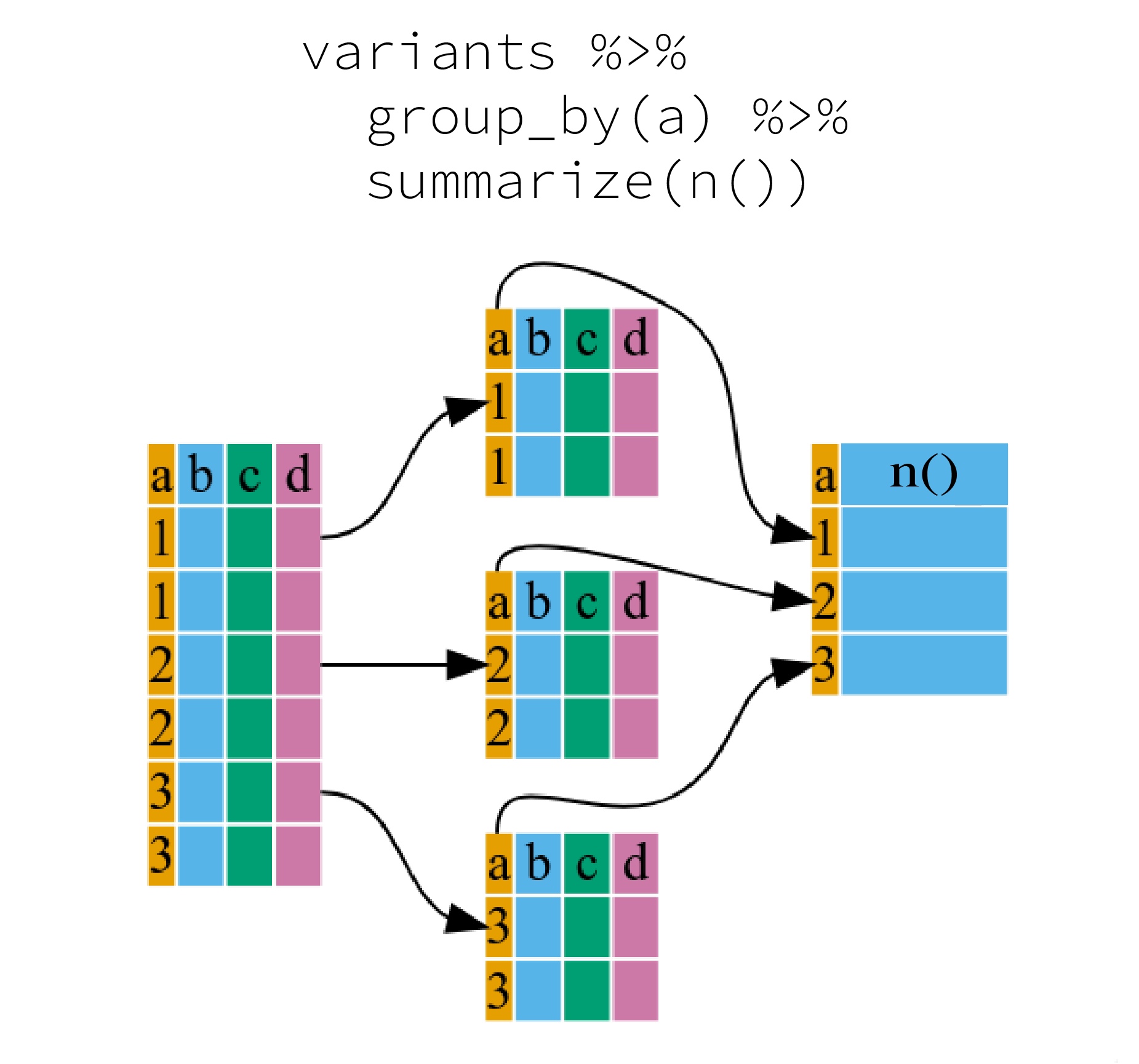
# ℹ 791 more rowsgroup_by() and summarize() functions
Many data analysis tasks can be approached using the
“split-apply-combine” paradigm: split the data into groups, apply some
analysis to each group, and then combine the results. dplyr
makes this very easy through the use of the group_by()
function, which splits the data into groups.
We can use group_by() to tally the number of mutations
detected in each sample using the function tally():
R
variants %>%
  group_by(sample_id) %>%
  tally()
OUTPUT
# A tibble: 3 × 2
  sample_id      n
  <chr>      <int>
1 SRR2584863    25
2 SRR2584866   766
3 SRR2589044    10
Since counting or tallying values is a common use case for
group_by(), an alternative function was created to bypasses
group_by() using the function count():
R
variants %>%
  count(sample_id)
OUTPUT
# A tibble: 3 × 2
  sample_id      n
  <chr>      <int>
1 SRR2584863    25
2 SRR2584866   766
3 SRR2589044    10
Challenge
- Count how many mutations are INDELS vs substitutions (aka not indels).
- Hint: INDELS is TRUE/FALSE column in the data.
R
variants %>%
  count(INDEL)
OUTPUT
# A tibble: 2 × 2
  INDEL     n
  <lgl> <int>
1 FALSE   700
2 TRUE    101
When the data is grouped, summarize() can be used to
collapse each group into a single-row summary. summarize()
does this by applying an aggregating or summary function to each
group.
It can be a bit tricky at first, but we can imagine physically splitting the data frame by groups and applying a certain function to summarize the data.
We can also apply many other functions to individual columns to get
other summary statistics. For example,we can use built-in functions like
mean(), median(), min(), and
max(). These are called “built-in functions” because they
come with R and don’t require that you install any additional packages.
By default, all R functions operating on vectors that contains
missing data will return NA. It’s a way to make sure that users
know they have missing data, and make a conscious decision on how to
deal with it. When dealing with simple statistics like the mean, the
easiest way to ignore NA (the missing data) is to use
na.rm = TRUE (rm stands for remove).
So to view the mean, median, maximum, and minimum filtered depth
(DP) for each sample:
R
variants %>%
  group_by(sample_id) %>%
  summarize(
    mean_DP = mean(DP),
    median_DP = median(DP),
    min_DP = min(DP),
    max_DP = max(DP))
OUTPUT
# A tibble: 3 × 5
  sample_id  mean_DP median_DP min_DP max_DP
  <chr>        <dbl>     <dbl>  <dbl>  <dbl>
1 SRR2584863    10.4      10        2     20
2 SRR2584866    10.6      10        2     79
3 SRR2589044 9.3 9.5 3 16Grouped Data Frames in Tidyverse
When you group a data frame with group_by(), you get a
grouped data frame. This is a special type of data frame that has all
the properties of a regular data frame but also has an additional
attribute that describes the grouping structure. The primary advantage
of a grouped data frame is that it allows you to work with each group of
observations as if they were a separate data frame.
Operations like summarise() and mutate()
will be applied to each group separately. This is particularly useful
when you want to perform calculations on subsets of your data.
To remove the grouping structure from a grouped data frame, you can
use the ungroup() function. This will return a regular data
frame.
For more details, refer to the dplyr documentation on grouping.
Combining data frames
There are times you may have multiple data tables that have information that could come together in them. This is often a structure set up that reflects database management where you you separate out different information into different related tables. For example, you may have one table that contains the results from your SNP analysis, as we have been using in this lesson, and another that has the metadata about your samples. For some applications you may want to pull information from that metadata table and be able to use it in your SNP analysis, maybe particular groupings that are repsented in the metadata table or alternate names, or other information.
For our example, we want to be able to use the generation number
instead of the sample_id for further analyses and perhaps
plotting later. We have a table of metadata from the Project
Organization and Management for Genomics lesson that includes
columns that matches up the sample_id column with the
generation information.
First, we will download the metadata table using the
download.file function in R.
R
download.file("https://raw.githubusercontent.com/datacarpentry/wrangling-genomics/gh-pages/files/Ecoli_metadata_composite.tsv", destfile = "data/Ecoli_metadata_composite.tsv")
We will only need to do this once and not every time we run our script so we can then comment the last line out.
Next we need to load the metadata table into an object in R. This
time we will use the read_delim() function as it has preset
arguments that work well for tab separated value files,
tsv, which is the format this table is
R
metadata <- read_delim("data/Ecoli_metadata_composite.tsv")
WARNING
Warning: One or more parsing issues, call `problems()` on your data frame for details,
e.g.:
  dat <- vroom(...)
  problems(dat)
This prints a warning message because the last entry is missing some values but it should still work for our purposes.
Before we match-up our table, we will simplify the metadata table to only include 3 columns.
R
metadata_sub <- select(metadata, strain, generation, run)
Now we need to consider how we want to merge these two tables together. There are many ways we might intersect these two tables, for example: Do we want an intersection that only keeps rows that match in a certain column from both tables? Do we want to keep only the rows from one table and the matching information from the other table? Do we want to keep only the non-matching information from both tables (though this is less common)?
In our case we want to keep all the rows from the
variants table and then pull information that matches from
the metadata_sub table. First, we will explore what happens
when we join these tables in other ways as well as an experiment.
First we will try to keep only the rows, observations, that match in
both tables. This is called an inner_join. For this join we
need to tell it which columns are equivalent in our two data frames. You
will not need to do this if the columns have the same name across data
frames but in our case what is called sample_id in the
variants data frame is called run in the
metadata_sub data frame.
R
inner <- inner_join(variants, metadata_sub, by = join_by(sample_id == run))
In this case the inner data frame is the same number of
rows (801) as the variants data frame. This is because all
of the sample_id’s that are in the variants
data frame have a corresponding run in
metadata_sub. If one was missing, then all of the data for
that sample would be dropped from the resulting data frame.
We can also see that instead of having 29 columns/variables like
variants, inner has 31 columns/variables. You
may want to run View(inner) and scroll to the far right to
see the new strain, and generation columns
that were added from the metadata_sub table. Note, it did
not add on the run column since that is repeated
information in the sample_id column. Also, we would have
had many more new columns added if we had used the full
metadata data frame instead of the
metadata_sub data frame.
Next we will try an “outer join” which only keeps all observations which are present in either data frames.
R
full <- full_join(variants, metadata_sub, by = join_by(sample_id == run))
The new full data frame now has more rows than
inner or variants! Though it has the same
number of columns as inner adding on the two additional
strain and generation columns. Why do you
think this has more rows than our original data? Hint: You may want
to View(full) and scroll down to the botton of the data
frame.
Once you look at the bottom of the data frame, you will see a bunch
of sample_id’s that we did not run the SNP analysis on but
were in the metadata_sub data frame. The full join will
keep every unique observation from your by columns even if
they do not match up in the other table.
This isn’t quite what we were looking for either.
What we want is to keep all the data in our variants
data frame, even if we do not find a match for it in the
metadata_sub table, so we avoid dropping any data if the
metadata_sub is missing some information. In this case we
will instead use another “outer join” option called “left join”. A left
join keeps all of the data in the table written on the left side of our
function, and will add on columns where the table on the right side
matches via our by statement.
R
# arguments      "left tbl"  "right tbl"
left <- left_join(variants, metadata_sub, by = join_by(sample_id == run))
In this case, the resulting data frame matches our inner
result exactly because there was no missing data in our right table.
Note: A “right” join is the opposite of a “left” so it will keep all the
data in the right most listed table and merge on the info in the left
most listed table
It is important to think carefully about what kind of join you want and check the resulting data frames to make sure they are what you expected when you planned your join. In this case, our “inner” and “left” join are the same but you want to be careful about possibly dropping or duplicating data depending on how the data frames are structured.
Finally, we can now do a data manipulation using the
generation column instead of the sample_id
column. We can repeat the calculations for counting SNPs for each
sample
R
left %>%
  count(generation)
OUTPUT
# A tibble: 3 × 2
  generation     n
       <dbl> <int>
1       5000    10
2      15000    25
3      50000   766
This result makes it easier to see the accumulation of more SNPs at later generations, without us having to know the sample IDs.
What about right joins?
- How many rows and columns would you expect from the following right join?
right_join(variants, metadata_sub, by = join_by(sample_id == run))
- How many rows and columns would you expect from the following right join?
right_join(metadata_sub, variants, by = join_by(run == sample_id))
Think carefully about the data in question and which data frame is on the right and which is on the left.
Part 1 There will be 860 rows and 31 variables, just
like the full join. All of the sample_id’s in the
variants data frame have matches and will be kept and then
it will also add on the run values that do not match but
were represented in the metadata_sub data frame with empty
info in the other columns since there is no matching rows in the
variants data frame.
Part 2 There will be 801 rows and 31 variables, just
like the inner and left joins. This join should always match exactly the
left join as it is the mirrored right join. It will only match the inner
join if all of the samples in the by match-up in the right
data frame are in the left data frame as well, otherwise it will drop
the rows not listed in the left for the inner join.
Reshaping data frames - Extra
It can sometimes be useful to transform the “long” tidy format, into
the wide format. This transformation can be done with the
pivot_wider() function provided by the tidyr
package (also part of the tidyverse).
pivot_wider() takes a data frame as the first argument,
and two arguments: the column name that will become the columns and the
column name that will become the cells in the wide data.
R
variants_wide <- variants %>%
  group_by(sample_id, CHROM) %>%
  summarize(mean_DP = mean(DP)) %>%
  pivot_wider(names_from = sample_id, values_from = mean_DP)
OUTPUT
`summarise()` has regrouped the output.
ℹ Summaries were computed grouped by sample_id and CHROM.
ℹ Output is grouped by sample_id.
ℹ Use `summarise(.groups = "drop_last")` to silence this message.
ℹ Use `summarise(.by = c(sample_id, CHROM))` for per-operation grouping
  (`?dplyr::dplyr_by`) instead.
R
variants_wide
OUTPUT
# A tibble: 1 × 4
  CHROM      SRR2584863 SRR2584866 SRR2589044
  <chr>           <dbl>      <dbl>      <dbl>
1 CP000819.1       10.4       10.6        9.3
The opposite operation of pivot_wider() is taken care by
pivot_longer(). We specify the names of the new columns,
and here add -CHROM as this column shouldn’t be affected by
the reshaping:
R
variants_wide %>%
  pivot_longer(-CHROM, names_to = "sample_id", values_to = "mean_DP")
OUTPUT
# A tibble: 3 × 3
  CHROM      sample_id  mean_DP
  <chr>      <chr>        <dbl>
1 CP000819.1 SRR2584863    10.4
2 CP000819.1 SRR2584866    10.6
3 CP000819.1 SRR2589044     9.3
Resources
- Use the
dplyrpackage to manipulate data frames. - Use
glimpse()to quickly look at your data frame. - Use
select()to choose variables from a data frame. - Use
filter()to choose data based on values. - Use
mutate()to create new variables. - Use
group_by()andsummarize()to work with subsets of data.
The figure was adapted from the Software Carpentry lesson, R for Reproducible Scientific Analysis↩︎