Introducing Scikit Learn
Overview
Teaching: 15 min
Exercises: 20 minQuestions
How can I use scikit-learn to process data?
Objectives
Recall that scikit-learn has built in linear regression functions.
Measure the error between a regression model and real data.
Apply scikit-learn’s linear regression to create a model.
Analyse and assess the accuracy of a linear model using scikit-learn’s metrics library.
Understand that more complex models can be built with non-linear equations.
Apply scikit-learn’s polynomial modelling to non-linear data.
SciKit Learn (also known as sklearn) is an open source machine learning library for Python which has a very wide range of machine learning algorithms. It makes it very easy for a Python programmer to use machine learning techniques without having to implement them.
Linear Regression with scikit-learn
Instead of coding least squares, an error function, and a model prediction function from scratch, we can use the Sklearn library to help us speed up our machine learning code development.
Let’s create an adapted copy of process_life_expectancy_data() called process_life_expectancy_data_sklearn(). We’ll replace our own functions (e.g., least_squares()) with Sklearn function calls.
Start by adding some additional Sklearn modules to the top of our regression_helper_functions.py file.
# Import modules from Sklearn library at top of .py file
import sklearn.linear_model as skl_lin # linear model
import sklearn.metrics as skl_metrics # error metrics
Next, locate the process_life_expectancy_data_sklearn() function in regression_helper_functions.py, and replace our custom functions with Sklearn function calls.
The scikit-learn regression function is much more capable than the simple one we wrote earlier and is designed for datasets where multiple parameters are used, its expecting to be given multi-demnsional arrays data. To get it to accept single dimension data such as we have we need to convert the array to a numpy one and use numpy’s reshape function. The resulting data is also designed to show us multiple coefficients and intercepts, so these values will be arrays, since we’ve just got one parameter we can just grab the first item from each of these arrays. Instead of manually calculating the results we can now use scikit-learn’s predict function. Finally lets calculate the error. scikit-learn doesn’t provide a root mean squared error function, but it does provide a mean squared error function. We can calculate the root mean squared error simply by taking the square root of the output of this function. The mean_squared_error function is part of the scikit-learn metrics module, so we’ll have to add that to our imports at the top of the file:
def process_life_expectancy_data_sklearn(filename, country, train_data_range, test_data_range=None):
    """Model and plot life expectancy over time for a specific country. Model is fit to data
    spanning train_data_range, and tested on data spanning test_data_range"""

    # Extract date range used for fitting the model
    min_date_train = train_data_range[0]
    max_date_train = train_data_range[1]

    # Read life expectancy data
    df = pd.read_csv(filename, index_col="Life expectancy")

    # get the data used to estimate line of best fit (life expectancy for specific
    # country across some date range)

    # we have to convert the dates to strings as pandas treats them that way
    y_train = df.loc[country, str(min_date_train):str(max_date_train)]

    # create a list with the numerical range of min_date to max_date
    # we could use the index of life_expectancy but it will be a string
    # we need numerical data
    x_train = list(range(min_date_train, max_date_train + 1))

    # NEW: Sklearn functions typically accept numpy arrays as input. This code will convert our list data into numpy arrays (N rows, 1 column)
    x_train = np.array(x_train).reshape(-1, 1)
    y_train = np.array(y_train).reshape(-1, 1)

    # OLD VERSION: m, c = least_squares([x_train, y_train])
    regression = None # FIXME: calculate line of best fit and extract m and c using sklearn.
    regression = skl_lin.LinearRegression().fit(x_train, y_train)

    # extract slope (m) and intercept (c)
    m = regression.coef_[0][0] # store coefs as (n_targets, n_features), where n_targets is the number of variables in Y, and n_features is the number of variables in X
    c = regression.intercept_[0]

    # print model parameters
    print("Results of linear regression:")
    print("m =", format(m,'.5f'), "c =", format(c,'.5f'))

    # OLD VERSION: y_train_pred = get_model_predictions(x_train, m, c)
    y_train_pred = None # FIXME: get model predictions for test data.
    y_train_pred = regression.predict(x_train)

    # OLD VERSION: train_error = measure_error(y_train, y_train_pred)
    train_error = None # FIXME: calculate model train set error.
    train_error = math.sqrt(skl_metrics.mean_squared_error(y_train, y_train_pred))

    print("Train RMSE =", format(train_error,'.5f'))
    if test_data_range is None:
        make_regression_graph(x_train.tolist(),
                              y_train.tolist(),
                              y_train_pred.tolist(),
                              ['Year', 'Life Expectancy'])

    # Test RMSE
    if test_data_range is not None:
        min_date_test = test_data_range[0]
        if len(test_data_range)==1:
            max_date_test=min_date_test
        else:
            max_date_test = test_data_range[1]
        x_test = list(range(min_date_test, max_date_test + 1))
        y_test = df.loc[country, str(min_date_test):str(max_date_test)]

        # convert data to numpy array
        x_test = np.array(x_test).reshape(-1, 1)
        y_test = np.array(y_test).reshape(-1, 1)

        # get predictions
        y_test_pred = regression.predict(x_test)

        # measure error
        test_error = math.sqrt(skl_metrics.mean_squared_error(y_test, y_test_pred))
        print("Test RMSE =", format(test_error,'.5f'))

        # plot train and test data along with line of best fit
        make_regression_graph(x_train.tolist(), y_train.tolist(), y_train_pred.tolist(),
                              ['Year', 'Life Expectancy'],
                              x_test.tolist(), y_test.tolist(), y_test_pred.tolist())

    return m, c
Now if we go ahead and run the new program we should get the same answers and same graph as before.
from regression_helper_functions import process_life_expectancy_data_sklearn

filepath = 'data/gapminder-life-expectancy.csv'
process_life_expectancy_data_sklearn(filepath,
                             "United Kingdom", [1950, 2010])

# Let's compare this result to our orginal implementation
process_life_expectancy_data(filepath,
                             "United Kingdom", [1950, 2010])
plt.show()
Polynomial regression
Linear regression obviously has its limits for working with data that isn’t linear. Scikit-learn has a number of other regression techniques which can be used on non-linear data. Some of these (such as isotonic regression) will only interpolate data in the range of the training data and can’t extrapolate beyond it. One non-linear technique that works with many types of data is polynomial regression. This creates a polynomial equation of the form y = a + bx + cx^2 + dx^3 etc. The more terms we add to the polynomial the more accurately we can model a system.
Scikit-learn includes a polynomial modelling tool as part of its pre-processing library which we’ll need to add to our list of imports.
- Add the following line of code to the top of regression_helper_functions():
import sklearn.preprocessing as skl_pre - Review the process_life_expectancy_data_poly() function and fix the FIXME tags
- Fit a linear model to a 5-degree polynomial transformation of x (dates). For a 5-degree polynomial applied to one feature (dates), we will get six new features or predictors: [1, x, x^2, x^3, x^4, x^5]
import sklearn.preprocessing as skl_pre
Fix the FIXME tags.
def process_life_expectancy_data_poly(degree: int,
                                      filename: str,
                                      country: str,
                                      train_data_range: Tuple[int, int],
                                      test_data_range: Optional[Tuple[int, int]] = None) -> None:
    """
    Model and plot life expectancy over time for a specific country using polynomial regression.

    Args:
        degree (int): The degree of the polynomial regression.
        filename (str): The CSV file containing the data.
        country (str): The name of the country for which the model is built.
        train_data_range (Tuple[int, int]): A tuple specifying the range of training data years (min_date, max_date).
        test_data_range (Optional[Tuple[int, int]]): A tuple specifying the range of test data years (min_date, max_date).

    Returns:
        None: The function displays plots but does not return a value.
    """

    # Extract date range used for fitting the model
    min_date_train = train_data_range[0]
    max_date_train = train_data_range[1]

    # Read life expectancy data
    df = pd.read_csv(filename, index_col="Life expectancy")

    # get the data used to estimate line of best fit (life expectancy for specific country across some date range)
    # we have to convert the dates to strings as pandas treats them that way
    y_train = df.loc[country, str(min_date_train):str(max_date_train)]

    # create a list with the numerical range of min_date to max_date
    # we could use the index of life_expectancy but it will be a string
    # we need numerical data
    x_train = list(range(min_date_train, max_date_train + 1))

    # This code will convert our list data into numpy arrays (N rows, 1 column)
    x_train = np.array(x_train).reshape(-1, 1)
    y_train = np.array(y_train).reshape(-1, 1)

    # Generate a new feature matrix consisting of all polynomial combinations of the features with degree less than or equal to the specified degree. For example, if an input sample is two dimensional and of the form [a, b], the degree-2 polynomial features are [1, a, b, a^2, ab, b^2].
    # for a 5-degree polynomial applied to one feature (dates), we will get six new features: [1, x, x^2, x^3, x^4, x^5]
    polynomial_features = None # FIXME: initialize polynomial features, [1, x, x^2, x^3, ...]
    polynomial_features = skl_pre.PolynomialFeatures(degree=degree)

    x_poly_train = None # FIXME:  apply polynomial transformation to training data
    x_poly_train = polynomial_features.fit_transform(x_train)

    print('x_train.shape', x_train.shape)
    print('x_poly_train.shape', x_poly_train.shape)

    # Calculate line of best fit using sklearn.
    regression = None # fit regression model
    regression = skl_lin.LinearRegression().fit(x_poly_train, y_train)

    # Get model predictions for test data
    y_train_pred = regression.predict(x_poly_train)

    # Calculate model train set error
    train_error = math.sqrt(skl_metrics.mean_squared_error(y_train, y_train_pred))

    print("Train RMSE =", format(train_error,'.5f'))
    if test_data_range is None:
        make_regression_graph(x_train.tolist(),
                              y_train.tolist(),
                              y_train_pred.tolist(),
                              ['Year', 'Life Expectancy'])

    # Test RMSE
    if test_data_range is not None:
        min_date_test = test_data_range[0]
        if len(test_data_range)==1:
            max_date_test=min_date_test
        else:
            max_date_test = test_data_range[1]

        # index data
        x_test = list(range(min_date_test, max_date_test + 1))
        y_test = df.loc[country, str(min_date_test):str(max_date_test)]

        # convert to numpy array
        x_test = np.array(x_test).reshape(-1, 1)
        y_test = np.array(y_test).reshape(-1, 1)

        # transform x data
        x_poly_test = polynomial_features.fit_transform(x_test)

        # get predictions on transformed data
        y_test_pred = regression.predict(x_poly_test)

        # measure error
        test_error = math.sqrt(skl_metrics.mean_squared_error(y_test, y_test_pred))
        print("Test RMSE =", format(test_error,'.5f'))

        # plot train and test data along with line of best fit
        make_regression_graph(x_train.tolist(), y_train.tolist(), y_train_pred.tolist(),
                              ['Year', 'Life Expectancy'],
                              x_test.tolist(), y_test.tolist(), y_test_pred.tolist())
Next, let’s fit a polynomial regression model of life expectancy in the UK between the years 1950 and 1980. How many predictor variables are used to predict life expectancy in this model? What do you notice about the plot? What happens if you decrease the degree of the polynomial?
There are 6 predictor variables in a 5-degree polynomial: [1, x, x^2, x^3, x^4, x^5]. The model appears to fit the data quite well when a 5-degree polynomial is used. As we decrease the degree of the polynomial, the model fits the training data less precisely.
from regression_helper_functions import process_life_expectancy_data_poly

filepath = 'data/gapminder-life-expectancy.csv'
process_life_expectancy_data_poly(5, filepath,
                             "United Kingdom", [1950, 1980])
plt.show()
Now let’s modify our call to process_life_expectancy_data_poly() to report the model’s ability to generalize to future data (left out during the model fitting/training process). What is the model’s test set RMSE for the time-span 2005:2016?
filepath = 'data/gapminder-life-expectancy.csv'
process_life_expectancy_data_poly(5, filepath,
                             "United Kingdom", [1950, 1980],[2005,2016])
plt.show()
The test RMSE is very high! Sometimes a more complicated model isn’t always a better model in terms of the model’s ability to generalize to unseen data. When a model fits training data well but poorly generalized to test data, we call this overfitting.
Let’s compare the polynomial model with our standard linear model.
process_life_expectancy_data_poly(10, filepath,
                             "United Kingdom", [1950, 1980],[2005,2016])
process_life_expectancy_data_sklearn(filepath,
                             "United Kingdom", [1950, 1980],[2005,2016])
plt.show()
Exercise: Comparing linear and polynomial models
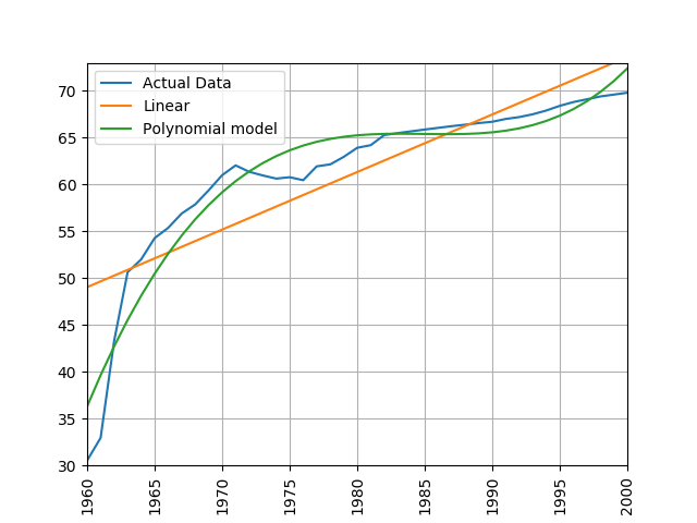
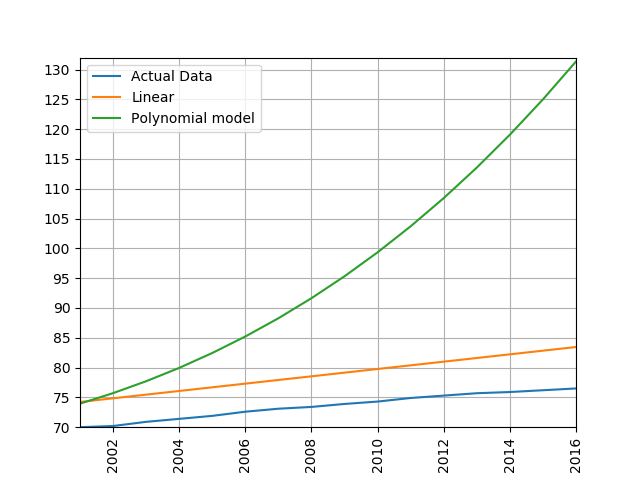
Train a linear and polynomial model on life expectancy data from China between 1960 and 2000. Then predict life expectancy from 2001 to 2016 using both methods. Compare their root mean squared errors, which is more accurate? Why do you think this model is the more accurate one?
Solution
modify the call to the process_life_expectancy_data
process_life_expectancy_data_poly("../data/gapminder-life-expectancy.csv", "China", 1960, 2000)linear prediction error is 5.385162846665607 polynomial prediction error is 28.169167771983528 The linear model is more accurate, polynomial models often become wildly inaccurate beyond the range they were trained on. Look at the predicted life expectancies, the polynomial model predicts a life expectancy of 131 by 2016!

Key Points
Scikit Learn is a Python library with lots of useful machine learning functions.
Scikit Learn includes a linear regression function.
It also includes a polynomial modelling function which is useful for modelling non-linear data.
