R for text data

Overview

Teaching: FIXME min
Exercises: FIXME min

Questions

FIXME

Objectives

FIXME

Why do this in R?

Data is rarely clean and tidy
Misspellings
White space
Multiple variables per column
Inconsistent coding
Fixing it by hand takes forever

Types of text data

Up until now, we’ve largely treated all text data the same as either all factors or all strings. However, the type of a text column in a tibble determines what you can do with the data. If you want to clean up misspellings or look for patterns in unstructured data, you can do that in a string column. If you want to subset based on a catagory or combine categories, factors are more useful.

This lesson will cover packages that make working with text data easier: stringr and forcats. These packages are part of the tidyverse, meaning that they work well with dplyr, specifically the mutate function. We will also cover options in the read_csv function that will allow you to choose what type the data are when they are imported.

Download Data

Link to download the data

Factors

Factors are categorical vectors in R. While some of the operations you can do on them are the same as with character vectors, others differ. They also different in their underlying structure. Character vectors are stored as the characters in each vector. Factors assign a value to each category and then store the values instead of the characters for each item. Given that this reduces the size of your data set, many functions may run faster when categories are set as factors instead of characters.

The data

We will be using a messier version of the surveys data that were used in the dplyr and ggplot2 lessons.

Importing the data

Let’s start by loading the libraries and importing the data with read_csv.

library(tidyverse)
# OR
library(stringr)
library(forcats)
library(ggplot2)
library(dplyr)
library(readr)
library(tidyr)

surveys<-read_csv(file = "data/Portal_rodents_19772002_scinameUUIDs.csv")

Warning: One or more parsing issues, call `problems()` on your data frame for details,
e.g.:
  dat <- vroom(...)
  problems(dat)

Rows: 35549 Columns: 39
── Column specification ────────────────────────────────────────────────────────
Delimiter: ","
chr (22): survey_id, plot_id, species, scientificName, locality, JSON, count...
dbl (16): recordID, mo, dy, yr, period, plot, note1, stake, decimalLatitude,...
lgl  (1): note3

ℹ Use `spec()` to retrieve the full column specification for this data.
ℹ Specify the column types or set `show_col_types = FALSE` to quiet this message.

Note that there are a few parsing errors. This error happens becaues read_csv looks at the first 1000 rows of each column and guess which type that column should be based on those entries. In our case there are a few entries at the bottom of the notes columns which don’t fit the type it guessed based on the first 1000 rows. We will add the guess_max argument to have read_csv check the whole column before it automatically chooses a type for that column.

surveys <- read_csv(file = "data/Portal_rodents_19772002_scinameUUIDs.csv", 
                  guess_max = 40000)

Rows: 35549 Columns: 39
── Column specification ────────────────────────────────────────────────────────
Delimiter: ","
chr (25): survey_id, plot_id, species, scientificName, locality, JSON, count...
dbl (14): recordID, mo, dy, yr, period, plot, note1, stake, decimalLatitude,...

ℹ Use `spec()` to retrieve the full column specification for this data.
ℹ Specify the column types or set `show_col_types = FALSE` to quiet this message.

Because we imported the data using read_csv, all of the non-numeric columns were converted to the character class. If we used read.csv, they would all be factors.

Challenge 1

Look at the data columns in the surveys dataset. Which columns should be converted to factors? Which should stay as text? Why?

Hint: should any numeric columns be factors?

Solution to Challenge 1

Changing column classes

#Create a text vector
species<-c("AB", "AS", "AS", "AB")
class(species)

[1] "character"

#convert it to factor
species<-as_factor(species)
species

[1] AB AS AS AB
Levels: AB AS

class(species)

[1] "factor"

#convert back to character
species<-as.character(species) 
class(species)

[1] "character"

surveys<- surveys%>%
  mutate(species = as_factor(species))

surveys$scientificName <- as_factor(surveys$scientificName)

Or, you could specify the types of all of your columns upon reading.

surveys<-read_csv(file = "data/Portal_rodents_19772002_scinameUUIDs.csv",
                  col_types = cols(col_character(), #survey_id
                                col_character(), #recordID
                                col_integer(),    #Month
                                col_integer(),    #day
                                col_integer(),    #year
                                col_double(),    #period
                                col_factor(), #plot_id
                                col_factor(), #plot
                                col_character(), #note1
                                col_character(), #stake
                                col_factor(), #species
                                col_factor(), #scientificName
                                col_character(), #locality
                                col_character(), #JSON
                                col_double(), #decimalLatitude
                                col_double(), #decimalLongitude
                                col_factor(), #county
                                col_factor(), #state
                                col_factor(), #country
                                col_factor(), #sex
                                col_factor(), #age
                                col_character(), #reprod
                                col_character(), #testes
                                col_character(), #vagina
                                col_character(), #pregnant
                                col_character(), #nippples
                                col_character(), #lactation
                                col_double(), #hfl
                                col_double(), #wgt
                                col_character(), #tag
                                col_character(), #note2
                                col_character(), #ltag
                                col_character(), #note3
                                col_character(), #prevrt
                                col_integer(), #prevlet
                                col_character(), #nestdir
                                col_integer(), #neststk
                                col_character(), #note4
                                col_character() #note5
                                )
                  )

Challenge 2

Convert the columns you identified in Challenge 1 to factors

Solution to Challenge 2

Fun with Factors

Recoding factors, fct_recode()
Reordering factors, fct_relevel()

Recoding factors

One common function we may need to perform is recoding the factors. In this case we may want to use the month names, instead of their numbers.

surveys$mo_abbv <- surveys$mo %>% as.factor() %>% 
  fct_recode(Jan='1', Feb='2', Mar='3', Apr='4', May='5', 
             Jun='6', Jul='7', Aug='8', Sep='9', Oct='10',
             Nov='11', Dec='12')
head(surveys)

# A tibble: 6 × 40
  survey_id   recor…¹    mo    dy    yr period plot_id plot  note1 stake species
  <chr>       <chr>   <int> <int> <int>  <dbl> <fct>   <fct> <chr> <chr> <fct>  
1 491ec41b-0… 6545        9    18  1982     62 4dc160… 13    13    36    AB     
2 f280bade-4… 5220        1    24  1982     54 dcbbd3… 20    13    27    AB     
3 2b1b4a8a-c… 18932       8     7  1991    162 1e87b1… 19    13    33    AS     
4 e98e66c4-5… 20588       1    24  1993    179 91829d… 12    13    41    AS     
5 768cdd0d-9… 7020       11    21  1982     63 f24f2d… 24    13    72    AH     
6 13851c71-0… 7645        4    16  1983     67 f24f2d… 24    13    21    AH     
# … with 29 more variables: scientificName <fct>, locality <chr>, JSON <chr>,
#   decimalLatitude <dbl>, decimalLongitude <dbl>, county <fct>, state <fct>,
#   country <fct>, sex <fct>, age <fct>, reprod <chr>, testes <chr>,
#   vagina <chr>, pregnant <chr>, nipples <chr>, lactation <chr>, hfl <dbl>,
#   wgt <dbl>, tag <chr>, note2 <chr>, ltag <chr>, note3 <chr>, prevrt <chr>,
#   prevlet <int>, nestdir <chr>, neststk <int>, note4 <chr>, note5 <chr>,
#   mo_abbv <fct>, and abbreviated variable name ¹​recordID

Easier way to do this.

Getting the month abbreviations recoded more easily. First let’s look at the first 6 months.

surveys$mo %>% head()

[1]  9  1  8  1 11  4

Now we can use the month.abb[] to get back the abbreviated names. (Still looking at only the first 6)

month.abb[surveys$mo] %>% head()

[1] "Sep" "Jan" "Aug" "Jan" "Nov" "Apr"

Challenge

Add a new column called mo_full onto the surveys data from that includes the full month name.

Shortcut hint: Check out what month.name[] does.

Solution to Challenge

surveys$mo_full <- surveys$mo %>% as.factor() %>% 
  fct_recode(January='1', Febuary='2', March='3', April='4', May='5', 
             June='6', July='7', August='8', September='9', October='10',
             November='11', December='12')

surveys$mo_full <- month.name[surveys$mo]

Reorder factors

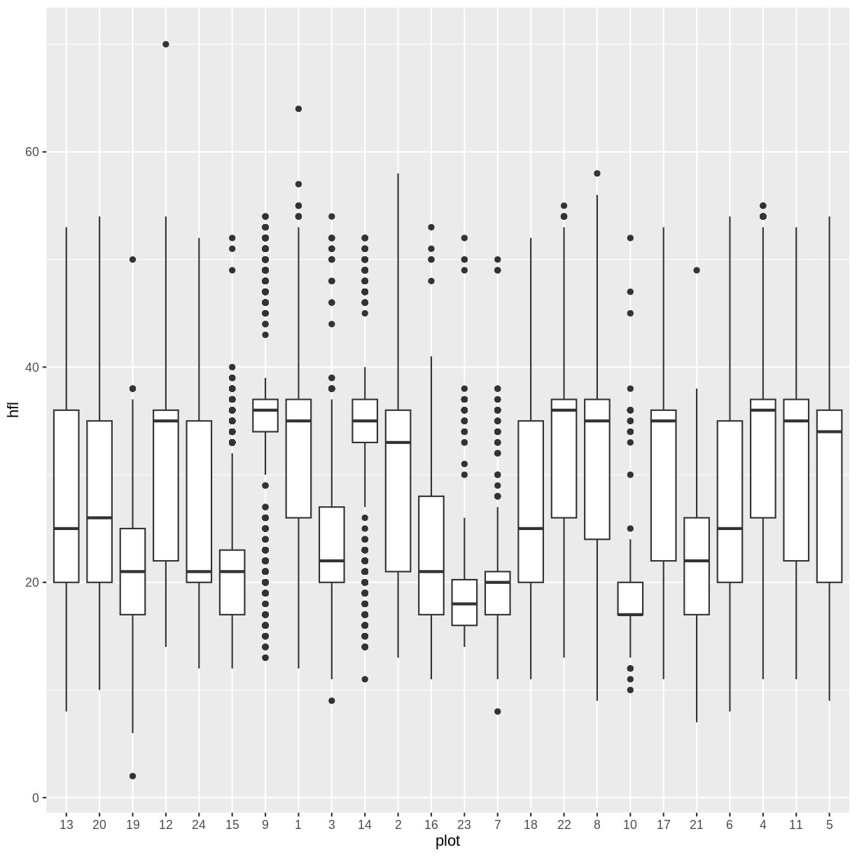
If we use the ggplot skills we learned in the last session. We see that the factors for plot_type display in the order of their levels, which are in alphabetical order by default.

levels(surveys$plot)

 [1] "13" "20" "19" "12" "24" "15" "9"  "1"  "3"  "14" "2"  "16" "23" "7"  "18"
[16] "22" "8"  "10" "17" "21" "6"  "4"  "11" "5" 

surveys %>% filter(!is.na(hfl)) %>% 
  ggplot(aes(x=plot, y=hfl)) +
  geom_boxplot()

plot of chunk unnamed-chunk-9

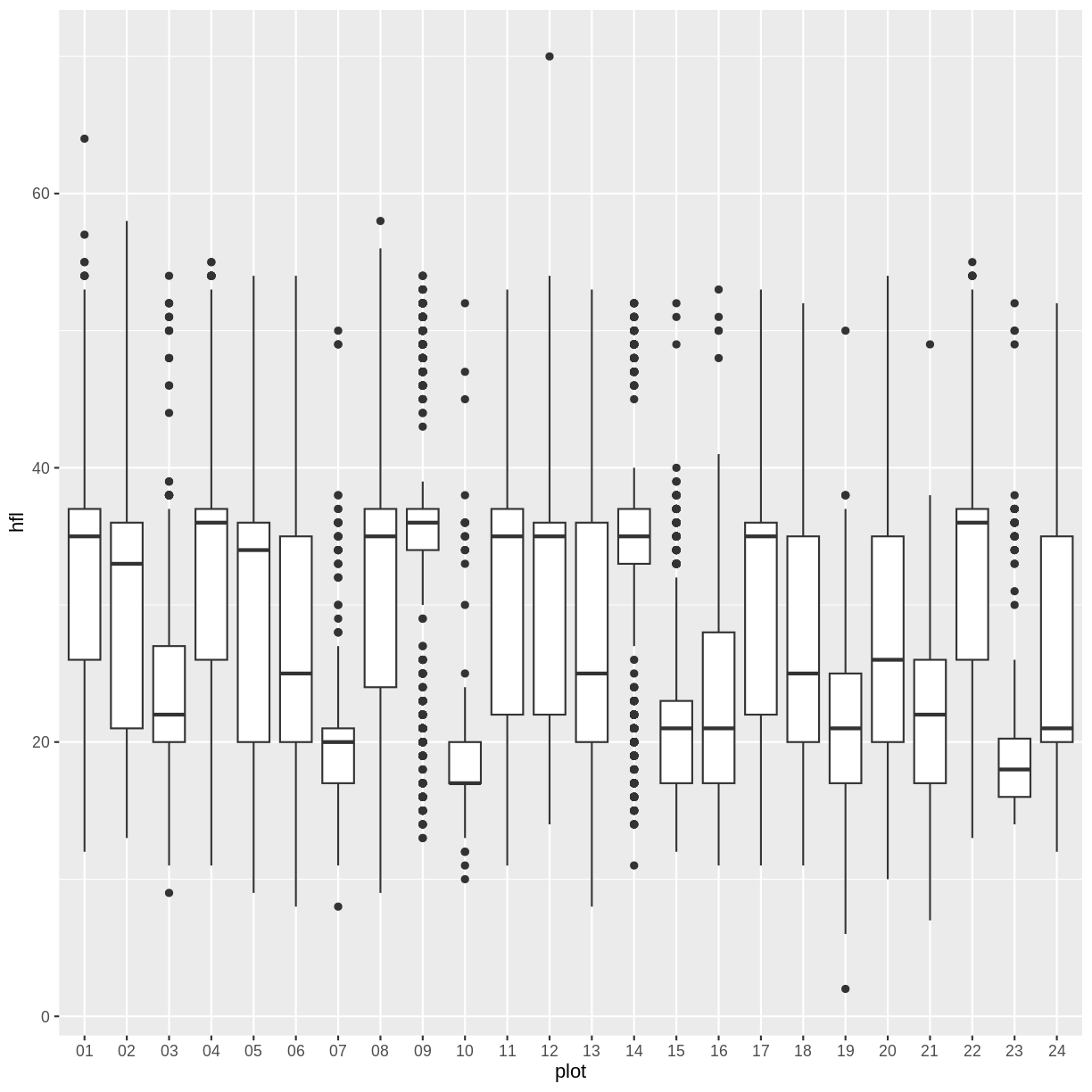
Ordered by number and left pad

Let’s put the plots in order by their number using the fct_relevel function.

surveys$plot %>% 
  levels() %>% 
  sort()

 [1] "1"  "10" "11" "12" "13" "14" "15" "16" "17" "18" "19" "2"  "20" "21" "22"
[16] "23" "24" "3"  "4"  "5"  "6"  "7"  "8"  "9" 

This sort is sorting alphabetically and by place. To fix the sorting, we can add a leading zero and ‘left pad’ the names using a string method.

str_pad(surveys$plot, width = 2, side = "left", pad="0") %>% head(10)

 [1] "13" "20" "19" "12" "24" "24" "15" "09" "15" "13"

surveys$plot <- str_pad(surveys$plot, width = 2, side = "left", pad="0") %>% as_factor()
order <- surveys$plot %>% 
  levels() %>%
  sort() 
surveys$plot <- fct_relevel(surveys$plot, order)
levels(surveys$plot)

 [1] "01" "02" "03" "04" "05" "06" "07" "08" "09" "10" "11" "12" "13" "14" "15"
[16] "16" "17" "18" "19" "20" "21" "22" "23" "24"

surveys %>% filter(!is.na(hfl)) %>% 
  ggplot(aes(x=plot, y=hfl)) +
  geom_boxplot()

plot of chunk unnamed-chunk-12

We can also reorder only a subset of the levels without having to specify all of the levels by using the after= argument We can say 1 (after the first level) to Inf (after everything) instead of typing out each of the levels in order.

We know from other information that the levels ‘2’, ‘4’, ‘8’, ‘11’, ‘12’, ‘17’, ‘22’ are the control plots. Let’s try putting the level ‘2’ at the end so we can see all the controls to the right.

surveys$plot <- surveys$plot %>% fct_relevel('2', after= Inf)

Warning: 1 unknown level in `f`: 2

Now if we plot the same box plot above, plot 2 is now on the far right. You can this to reorder the categories in other plots as well.

surveys %>% 
  filter(!is.na(hfl)) %>% 
  ggplot(aes(x=plot, y=hfl)) +
  geom_boxplot()

plot of chunk unnamed-chunk-14

Challenge

Reorder the plot’s in the boxplot above so all the control plots are on the right.

Solution to Challenge

surveys$plot<- surveys$plot %>% fct_relevel('2', '4', '8', '11', '12', '17', '22', after= Inf)
surveys %>% 
    filter(!is.na(hfl)) %>% 
    ggplot(aes(x=plot, y=hfl)) +
    geom_boxplot()

Cleaning up text data

When text data is entered by hand, small differences can be introduced that aren’t easy to see with the human eye, but are important to the computer. One easy way to identify these small differences is the count function.

surveys%>%
  count(scientificName)

# A tibble: 27 × 2
   scientificName                n
   <fct>                     <int>
Amphispiza bilineata        291
Ammodramus savannarum         2
Ammospermophilis harrisi      1
Ammospermophilus harrisi    435
Ammospermophilus harrisii     1
Amphespiza bilineata          7
Amphispiza bilineatus         1
Amphispiza cilineata          1
Amphispizo bilineata          1
Baiomys taylori              46
# … with 17 more rows

You can see some very similar species names, for example: “Ammospermophilis harrisi”, “Ammospermophilus harrisi”, “Ammospermophilus harrisii”. However one spelling has many more records than the others. How can we fix the spellings?

surveys$scientificName <- fct_explicit_na(surveys$scientificName)
surveys$scientificName <- fct_collapse(surveys$scientificName,
            "Ammospermophilus harrisi"=c("Ammospermophilus harrisi",
                                         "Ammospermophilis harrisi",
                                         "Ammospermophilus harrisii"),
            "Amphespiza bilineata" = c("Amphispiza bilineatus",
                                       "Amphispiza cilineata",
                                       "Amphispizo bilineata"))

We can see the change by looking at the count again.

surveys%>%
  count(scientificName)

# A tibble: 22 × 2
   scientificName                      n
   <fct>                           <int>
Amphispiza bilineata              291
Ammodramus savannarum               2
Ammospermophilus harrisi          437
Amphespiza bilineata               10
Baiomys taylori                    46
Calamospiza melanocorys             1
Callipepla squamata                 1
Campylorhynchus brunneicapillus     1
Chaetodipus baileyi                 2
Cnemidophorus tigris                1
# … with 12 more rows

Challenge

Find all the possible variants on the country name “United States””
Change them all to the most common variant.

Solution to Challenge

surveys %>% count(country)
# We can see that "United States of America", "UNITED STATES", and "US"
# Are possible options with "UNITED STATES" being the most common.
surveys$country <- fct_collapse(surveys$country, 
             "UNITED STATES" = c("United States of America",
                                 "US"))

Splitting Variables

Next we may want to split the scientific names into genus and species columns as we have seen in the cleaned version of the data.

surveys <- separate(surveys, scientificName, c("genusName", "speciesName"), sep="\\s", remove = FALSE)

Warning in gregexpr(pattern, x, perl = TRUE): PCRE error
	'UTF-8 error: isolated byte with 0x80 bit set'
	for element 16923

Warning in gregexpr(pattern, x, perl = TRUE): PCRE error
	'UTF-8 error: isolated byte with 0x80 bit set'
	for element 16924

Warning in gregexpr(pattern, x, perl = TRUE): PCRE error
	'UTF-8 error: isolated byte with 0x80 bit set'
	for element 16925

Warning in gregexpr(pattern, x, perl = TRUE): PCRE error
	'UTF-8 error: isolated byte with 0x80 bit set'
	for element 16926

Warning in gregexpr(pattern, x, perl = TRUE): PCRE error
	'UTF-8 error: isolated byte with 0x80 bit set'
	for element 16927

Warning in gregexpr(pattern, x, perl = TRUE): PCRE error
	'UTF-8 error: isolated byte with 0x80 bit set'
	for element 16928

Warning in gregexpr(pattern, x, perl = TRUE): PCRE error
	'UTF-8 error: isolated byte with 0x80 bit set'
	for element 16929

Warning in gregexpr(pattern, x, perl = TRUE): PCRE error
	'UTF-8 error: isolated byte with 0x80 bit set'
	for element 16930

Warning in gregexpr(pattern, x, perl = TRUE): PCRE error
	'UTF-8 error: isolated byte with 0x80 bit set'
	for element 16931

Warning in gregexpr(pattern, x, perl = TRUE): PCRE error
	'UTF-8 error: isolated byte with 0x80 bit set'
	for element 16932

Warning in gregexpr(pattern, x, perl = TRUE): PCRE error
	'UTF-8 error: isolated byte with 0x80 bit set'
	for element 16933

Warning in gregexpr(pattern, x, perl = TRUE): PCRE error
	'UTF-8 error: isolated byte with 0x80 bit set'
	for element 16934

Warning in gregexpr(pattern, x, perl = TRUE): PCRE error
	'UTF-8 error: isolated byte with 0x80 bit set'
	for element 16935

Warning in gregexpr(pattern, x, perl = TRUE): PCRE error
	'UTF-8 error: isolated byte with 0x80 bit set'
	for element 16936

Warning in gregexpr(pattern, x, perl = TRUE): PCRE error
	'UTF-8 error: isolated byte with 0x80 bit set'
	for element 16937

Warning in gregexpr(pattern, x, perl = TRUE): PCRE error
	'UTF-8 error: isolated byte with 0x80 bit set'
	for element 16938

Warning in gregexpr(pattern, x, perl = TRUE): PCRE error
	'UTF-8 error: isolated byte with 0x80 bit set'
	for element 16939

Warning in gregexpr(pattern, x, perl = TRUE): PCRE error
	'UTF-8 error: isolated byte with 0x80 bit set'
	for element 16940

Warning in gregexpr(pattern, x, perl = TRUE): PCRE error
	'UTF-8 error: isolated byte with 0x80 bit set'
	for element 16941

Warning in gregexpr(pattern, x, perl = TRUE): PCRE error
	'UTF-8 error: isolated byte with 0x80 bit set'
	for element 16942

Warning in gregexpr(pattern, x, perl = TRUE): PCRE error
	'UTF-8 error: isolated byte with 0x80 bit set'
	for element 16943

Warning in gregexpr(pattern, x, perl = TRUE): PCRE error
	'UTF-8 error: isolated byte with 0x80 bit set'
	for element 16944

Warning in gregexpr(pattern, x, perl = TRUE): PCRE error
	'UTF-8 error: isolated byte with 0x80 bit set'
	for element 16945

Warning in gregexpr(pattern, x, perl = TRUE): PCRE error
	'UTF-8 error: isolated byte with 0x80 bit set'
	for element 16946

Warning in gregexpr(pattern, x, perl = TRUE): PCRE error
	'UTF-8 error: isolated byte with 0x80 bit set'
	for element 16947

Warning in gregexpr(pattern, x, perl = TRUE): PCRE error
	'UTF-8 error: isolated byte with 0x80 bit set'
	for element 16948

Warning in gregexpr(pattern, x, perl = TRUE): PCRE error
	'UTF-8 error: isolated byte with 0x80 bit set'
	for element 16949

Warning in gregexpr(pattern, x, perl = TRUE): PCRE error
	'UTF-8 error: isolated byte with 0x80 bit set'
	for element 16950

Warning in gregexpr(pattern, x, perl = TRUE): PCRE error
	'UTF-8 error: isolated byte with 0x80 bit set'
	for element 16951

Warning in gregexpr(pattern, x, perl = TRUE): PCRE error
	'UTF-8 error: isolated byte with 0x80 bit set'
	for element 16952

Warning in gregexpr(pattern, x, perl = TRUE): PCRE error
	'UTF-8 error: isolated byte with 0x80 bit set'
	for element 16953

Warning in gregexpr(pattern, x, perl = TRUE): PCRE error
	'UTF-8 error: isolated byte with 0x80 bit set'
	for element 16954

Warning in gregexpr(pattern, x, perl = TRUE): PCRE error
	'UTF-8 error: isolated byte with 0x80 bit set'
	for element 16955

Warning in gregexpr(pattern, x, perl = TRUE): PCRE error
	'UTF-8 error: isolated byte with 0x80 bit set'
	for element 16956

Warning in gregexpr(pattern, x, perl = TRUE): PCRE error
	'UTF-8 error: isolated byte with 0x80 bit set'
	for element 16957

Warning in gregexpr(pattern, x, perl = TRUE): PCRE error
	'UTF-8 error: isolated byte with 0x80 bit set'
	for element 16958

Warning in gregexpr(pattern, x, perl = TRUE): PCRE error
	'UTF-8 error: isolated byte with 0x80 bit set'
	for element 16959

Warning in gregexpr(pattern, x, perl = TRUE): PCRE error
	'UTF-8 error: isolated byte with 0x80 bit set'
	for element 16960

Warning in gregexpr(pattern, x, perl = TRUE): PCRE error
	'UTF-8 error: isolated byte with 0x80 bit set'
	for element 16961

Warning in gregexpr(pattern, x, perl = TRUE): PCRE error
	'UTF-8 error: isolated byte with 0x80 bit set'
	for element 16962

Warning in gregexpr(pattern, x, perl = TRUE): PCRE error
	'UTF-8 error: isolated byte with 0x80 bit set'
	for element 20220

Warning in gregexpr(pattern, x, perl = TRUE): PCRE error
	'UTF-8 error: isolated byte with 0x80 bit set'
	for element 20221

Warning in gregexpr(pattern, x, perl = TRUE): PCRE error
	'UTF-8 error: isolated byte with 0x80 bit set'
	for element 20222

Warning in gregexpr(pattern, x, perl = TRUE): PCRE error
	'UTF-8 error: isolated byte with 0x80 bit set'
	for element 20223

Warning in gregexpr(pattern, x, perl = TRUE): PCRE error
	'UTF-8 error: isolated byte with 0x80 bit set'
	for element 20224

Warning in gregexpr(pattern, x, perl = TRUE): PCRE error
	'UTF-8 error: isolated byte with 0x80 bit set'
	for element 20225

Warning in gregexpr(pattern, x, perl = TRUE): PCRE error
	'UTF-8 error: isolated byte with 0x80 bit set'
	for element 20226

Warning in gregexpr(pattern, x, perl = TRUE): PCRE error
	'UTF-8 error: isolated byte with 0x80 bit set'
	for element 20227

Warning in gregexpr(pattern, x, perl = TRUE): PCRE error
	'UTF-8 error: isolated byte with 0x80 bit set'
	for element 20228

Warning in gregexpr(pattern, x, perl = TRUE): PCRE error
	'UTF-8 error: isolated byte with 0x80 bit set'
	for element 20229

Warning in gregexpr(pattern, x, perl = TRUE): PCRE error
	'UTF-8 error: isolated byte with 0x80 bit set'
	for element 20230

Warning in gregexpr(pattern, x, perl = TRUE): PCRE error
	'UTF-8 error: isolated byte with 0x80 bit set'
	for element 20231

Warning: Expected 2 pieces. Missing pieces filled with `NA` in 15370 rows [16923, 16924,
16925, 16926, 16927, 16928, 16929, 16930, 16931, 16932, 16933, 16934, 16935,
16936, 16937, 16938, 16939, 16940, 16941, 16942, ...].

Joining Variables

In some of our plots we may want to label with the full scientific name. To do so we can add a new column which joins two strings together. Before we get into vectors lets try an example with two strings

name = "Sarah"
str_c("Hi my name is ", name)

[1] "Hi my name is Sarah"

We can similarly use this on vectors. We can make one column that has the latitude and longitude.

surveys$latnlong <- str_c(surveys$decimalLatitude, " ",  surveys$decimalLongitude)

Another function that you could have used here is paste()

Other stringr functions

Next, let’s see if all our recordIDs are the same length.

str_length(surveys$recordID) %>%  head()

[1] 4 4 5 5 4 4

We can see that they are not all the same length but it is hard to see what the different lengths are lets see the different lengths using the unique() function.

str_length(surveys$recordID) %>% unique()

[1] 4 5 1 2 3

Challenge

Use the use stringr function we learned earlier to make all the recordIDs the same length.
Solution to Challenge
surveys$recordID<- surveys$recordID %>%  str_pad(width = 5, side = "left", pad = "0")

Another string function we can use is to get a subset of a string. We can use that function, str_sub() to create abbvs for the genera. We can then add those abbrvs as their own column

str_sub(surveys$genusName, 1, 5) %>%  head()

[1] "Amphi" "Amphi" "Ammod" "Ammod" "Ammos" "Ammos"

surveys <- surveys %>%  mutate(genusAbbv = str_sub(surveys$genusName, 1, 5))

Finding patterns

Rstudio Regular expression Cheatsheet Rstudio stingr Cheatsheet

Find the scientific names with punctuation in them.

str_detect(surveys$scientificName, "Dip") %>% head()

[1] FALSE FALSE FALSE FALSE FALSE FALSE

str_detect(surveys$scientificName, "Dip") %>% unique()

[1] FALSE  TRUE

str_subset(surveys$scientificName, "Dip") %>% head()

[1] "Dipodomys merriami" "Dipodomys merriami" "Dipodomys merriami"
[4] "Dipodomys merriami" "Dipodomys merriami" "Dipodomys merriami"

str_subset(surveys$scientificName, "Dip") %>% unique()

[1] "Dipodomys merriami"    "Dipodomys ordii"       "Dipodomys spectabilis"
[4] "Dipodomys�sp."        

str_subset(surveys$scientificName, "[[:punct:]]") %>% head()

[1] "Dipodomys�sp." "Dipodomys�sp." "Dipodomys�sp." "Dipodomys�sp."
[5] "Dipodomys�sp." "Dipodomys�sp."

str_subset(surveys$scientificName, "[[:punct:]]") %>% unique()

[1] "Dipodomys�sp." "Onychomys�sp." "(Missing)"

Let’s replace all the puntuation characters with a space for the moment.

statement = "Sarah is the instructor"
str_replace(statement, "a", "e")

[1] "Serah is the instructor"

str_replace_all(statement, "a", "e")

[1] "Sereh is the instructor"

surveys$scientificName <- str_replace_all(surveys$scientificName, "[[:punct:]]", " ")
surveys %>% count(scientificName)

# A tibble: 22 × 2
   scientificName                        n
   <chr>                             <int>
" Missing "                       15318
"Ammodramus savannarum"               2
"Ammospermophilus harrisi"          437
"Amphespiza bilineata"               10
"Amphispiza bilineata"              291
"Baiomys taylori"                    46
"Calamospiza melanocorys"             1
"Callipepla squamata"                 1
"Campylorhynchus brunneicapillus"     1
"Chaetodipus baileyi"                 2
# … with 12 more rows

Other pattern matching commands that can be useful:

str_match()
str_count()
str_locate()
str_extract()

Remove leading/trailing whitespace

Now we have some extra whitespace to remove from the scientificName column. We can use the str_trim function

str_subset(surveys$scientificName, "Miss") %>%  head()

[1] " Missing " " Missing " " Missing " " Missing " " Missing " " Missing "

str_subset(surveys$scientificName, "Miss")[1] %>% str_trim()

[1] "Missing"

str_trim(surveys$scientificName) %>% str_subset("Miss") %>%  head()

[1] "Missing" "Missing" "Missing" "Missing" "Missing" "Missing"

surveys$scientificName <- str_trim(surveys$scientificName)

Write back to a csv file

write_csv(surveys, "cleaned_surveys_20191005_slr.csv")

Key Points

FIXME

lesson home

UW Custom R Lesson

next episode

R for text data

Overview

Why do this in R?

Types of text data

Download Data

Factors

The data

Importing the data

Challenge 1

Solution to Challenge 1

Changing column classes

Challenge 2

Solution to Challenge 2

Fun with Factors

Recoding factors

Easier way to do this.

Challenge

Solution to Challenge

Reorder factors

Ordered by number and left pad

Challenge

Solution to Challenge

Cleaning up text data

Challenge

Solution to Challenge

Splitting Variables

Joining Variables

Other stringr functions

Challenge

Solution to Challenge

Finding patterns

Remove leading/trailing whitespace

Write back to a csv file

Key Points

lesson home

next episode