R for text data

Overview

Teaching: FIXME min
Exercises: FIXME min

Questions

• FIXME

Objectives

• FIXME

Why do this in R?

• Data is rarely clean and tidy
• Misspellings
• White space
• Multiple variables per column
• Inconsistent coding
• Fixing it by hand takes forever

Types of text data

Up until now, we’ve largely treated all text data the same as either all factors or all strings. However, the type of a text column in a tibble determines what you can do with the data. If you want to clean up misspellings or look for patterns in unstructured data, you can do that in a string column. If you want to subset based on a catagory or combine categories, factors are more useful.

This lesson will cover packages that make working with text data easier: stringr and forcats. These packages are part of the tidyverse, meaning that they work well with dplyr, specifically the mutate function. We will also cover options in the read_csv function that will allow you to choose what type the data are when they are imported.

Download Data

Link to download the data

Factors

Factors are categorical vectors in R. While some of the operations you can do on them are the same as with character vectors, others differ. They also different in their underlying structure. Character vectors are stored as the characters in each vector. Factors assign a value to each category and then store the values instead of the characters for each item. Given that this reduces the size of your data set, many functions may run faster when categories are set as factors instead of characters.

The data

We will be using a messier version of the surveys data that were used in the dplyr and ggplot2 lessons.

Importing the data

Let’s start by loading the libraries and importing the data with read_csv.

library(tidyverse)
# OR
library(stringr)
library(forcats)
library(ggplot2)
library(dplyr)
library(readr)
library(tidyr)

surveys<-read_csv(file = "data/Portal_rodents_19772002_scinameUUIDs.csv")

Warning: One or more parsing issues, call `problems()` on your data frame for details,
e.g.:
  dat <- vroom(...)
  problems(dat)

Rows: 35549 Columns: 39
── Column specification ────────────────────────────────────────────────────────
Delimiter: ","
chr (22): survey_id, plot_id, species, scientificName, locality, JSON, count...
dbl (16): recordID, mo, dy, yr, period, plot, note1, stake, decimalLatitude,...
lgl  (1): note3

ℹ Use `spec()` to retrieve the full column specification for this data.
ℹ Specify the column types or set `show_col_types = FALSE` to quiet this message.

Note that there are a few parsing errors. This error happens becaues read_csv looks at the first 1000 rows of each column and guess which type that column should be based on those entries. In our case there are a few entries at the bottom of the notes columns which don’t fit the type it guessed based on the first 1000 rows. We will add the guess_max argument to have read_csv check the whole column before it automatically chooses a type for that column.

surveys <- read_csv(file = "data/Portal_rodents_19772002_scinameUUIDs.csv", 
                  guess_max = 40000)

Rows: 35549 Columns: 39
── Column specification ────────────────────────────────────────────────────────
Delimiter: ","
chr (25): survey_id, plot_id, species, scientificName, locality, JSON, count...
dbl (14): recordID, mo, dy, yr, period, plot, note1, stake, decimalLatitude,...

ℹ Use `spec()` to retrieve the full column specification for this data.
ℹ Specify the column types or set `show_col_types = FALSE` to quiet this message.

Because we imported the data using read_csv, all of the non-numeric columns were converted to the character class. If we used read.csv, they would all be factors.

Challenge 1

Look at the data columns in the surveys dataset. Which columns should be converted to factors? Which should stay as text? Why?

Hint: should any numeric columns be factors?

Solution to Challenge 1

Changing column classes

#Create a text vector
species<-c("AB", "AS", "AS", "AB")
class(species)

[1] "character"

#convert it to factor
species<-as_factor(species)
species

[1] AB AS AS AB
Levels: AB AS

class(species)

[1] "factor"

#convert back to character
species<-as.character(species) 
class(species)

[1] "character"

surveys<- surveys%>%
  mutate(species = as_factor(species))

OR

surveys$scientificName <- as_factor(surveys$scientificName)

Or, you could specify the types of all of your columns upon reading.

surveys<-read_csv(file = "data/Portal_rodents_19772002_scinameUUIDs.csv",
                  col_types = cols(col_character(), #survey_id
                                col_character(), #recordID
                                col_integer(),    #Month
                                col_integer(),    #day
                                col_integer(),    #year
                                col_double(),    #period
                                col_factor(), #plot_id
                                col_factor(), #plot
                                col_character(), #note1
                                col_character(), #stake
                                col_factor(), #species
                                col_factor(), #scientificName
                                col_character(), #locality
                                col_character(), #JSON
                                col_double(), #decimalLatitude
                                col_double(), #decimalLongitude
                                col_factor(), #county
                                col_factor(), #state
                                col_factor(), #country
                                col_factor(), #sex
                                col_factor(), #age
                                col_character(), #reprod
                                col_character(), #testes
                                col_character(), #vagina
                                col_character(), #pregnant
                                col_character(), #nippples
                                col_character(), #lactation
                                col_double(), #hfl
                                col_double(), #wgt
                                col_character(), #tag
                                col_character(), #note2
                                col_character(), #ltag
                                col_character(), #note3
                                col_character(), #prevrt
                                col_integer(), #prevlet
                                col_character(), #nestdir
                                col_integer(), #neststk
                                col_character(), #note4
                                col_character() #note5
                                )
                  )

Challenge 2

Convert the columns you identified in Challenge 1 to factors

Solution to Challenge 2

Fun with Factors

• Recoding factors, fct_recode()
• Reordering factors, fct_relevel()

Recoding factors

One common function we may need to perform is recoding the factors. In this case we may want to use the month names, instead of their numbers.

surveys$mo_abbv <- surveys$mo %>% as.factor() %>% 
  fct_recode(Jan='1', Feb='2', Mar='3', Apr='4', May='5', 
             Jun='6', Jul='7', Aug='8', Sep='9', Oct='10',
             Nov='11', Dec='12')
head(surveys)

# A tibble: 6 × 40
  survey_id   recor…¹    mo    dy    yr period plot_id plot  note1 stake species
  <chr>       <chr>   <int> <int> <int>  <dbl> <fct>   <fct> <chr> <chr> <fct>  
1 491ec41b-0… 6545        9    18  1982     62 4dc160… 13    13    36    AB     
2 f280bade-4… 5220        1    24  1982     54 dcbbd3… 20    13    27    AB     
3 2b1b4a8a-c… 18932       8     7  1991    162 1e87b1… 19    13    33    AS     
4 e98e66c4-5… 20588       1    24  1993    179 91829d… 12    13    41    AS     
5 768cdd0d-9… 7020       11    21  1982     63 f24f2d… 24    13    72    AH     
6 13851c71-0… 7645        4    16  1983     67 f24f2d… 24    13    21    AH     
# … with 29 more variables: scientificName <fct>, locality <chr>, JSON <chr>,
#   decimalLatitude <dbl>, decimalLongitude <dbl>, county <fct>, state <fct>,
#   country <fct>, sex <fct>, age <fct>, reprod <chr>, testes <chr>,
#   vagina <chr>, pregnant <chr>, nipples <chr>, lactation <chr>, hfl <dbl>,
#   wgt <dbl>, tag <chr>, note2 <chr>, ltag <chr>, note3 <chr>, prevrt <chr>,
#   prevlet <int>, nestdir <chr>, neststk <int>, note4 <chr>, note5 <chr>,
#   mo_abbv <fct>, and abbreviated variable name ¹​recordID

Easier way to do this.

Getting the month abbreviations recoded more easily. First let’s look at the first 6 months.

surveys$mo %>% head()

[1]  9  1  8  1 11  4

Now we can use the month.abb[] to get back the abbreviated names. (Still looking at only the first 6)

month.abb[surveys$mo] %>% head()

[1] "Sep" "Jan" "Aug" "Jan" "Nov" "Apr"

Challenge

Add a new column called mo_full onto the surveys data from that includes the full month name.

Shortcut hint: Check out what month.name[] does.

Solution to Challenge

surveys$mo_full <- surveys$mo %>% as.factor() %>% 
  fct_recode(January='1', Febuary='2', March='3', April='4', May='5', 
             June='6', July='7', August='8', September='9', October='10',
             November='11', December='12')

OR

surveys$mo_full <- month.name[surveys$mo]

Reorder factors

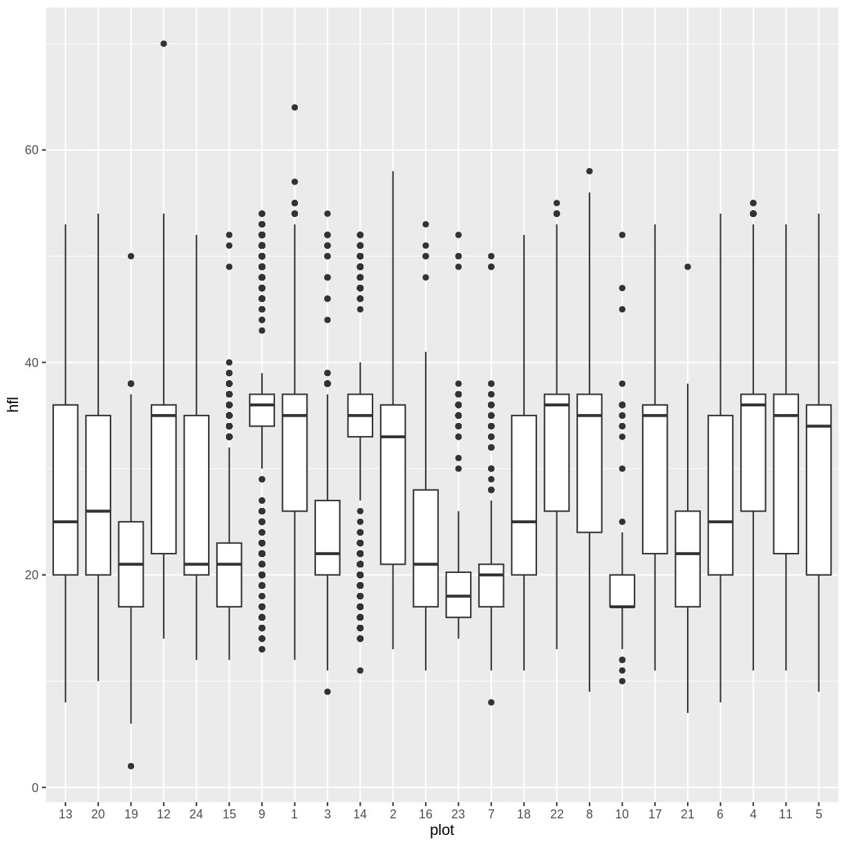
If we use the ggplot skills we learned in the last session. We see that the factors for plot_type display in the order of their levels, which are in alphabetical order by default.

levels(surveys$plot)

 [1] "13" "20" "19" "12" "24" "15" "9"  "1"  "3"  "14" "2"  "16" "23" "7"  "18"
[16] "22" "8"  "10" "17" "21" "6"  "4"  "11" "5" 

surveys %>% filter(!is.na(hfl)) %>% 
  ggplot(aes(x=plot, y=hfl)) +
  geom_boxplot()

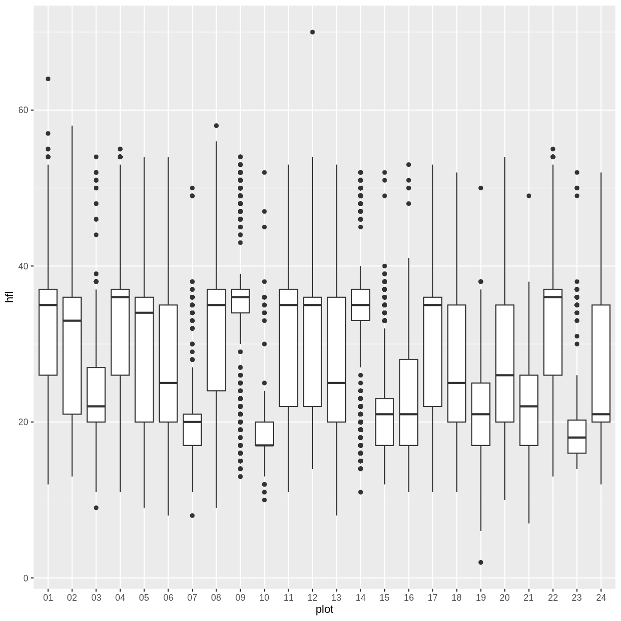
Ordered by number and left pad

Let’s put the plots in order by their number using the fct_relevel function.

surveys$plot %>% 
  levels() %>% 
  sort()

 [1] "1"  "10" "11" "12" "13" "14" "15" "16" "17" "18" "19" "2"  "20" "21" "22"
[16] "23" "24" "3"  "4"  "5"  "6"  "7"  "8"  "9" 

This sort is sorting alphabetically and by place. To fix the sorting, we can add a leading zero and ‘left pad’ the names using a string method.

str_pad(surveys$plot, width = 2, side = "left", pad="0") %>% head(10)

 [1] "13" "20" "19" "12" "24" "24" "15" "09" "15" "13"

surveys$plot <- str_pad(surveys$plot, width = 2, side = "left", pad="0") %>% as_factor()
order <- surveys$plot %>% 
  levels() %>%
  sort() 
surveys$plot <- fct_relevel(surveys$plot, order)
levels(surveys$plot)

 [1] "01" "02" "03" "04" "05" "06" "07" "08" "09" "10" "11" "12" "13" "14" "15"
[16] "16" "17" "18" "19" "20" "21" "22" "23" "24"

surveys %>% filter(!is.na(hfl)) %>% 
  ggplot(aes(x=plot, y=hfl)) +
  geom_boxplot()

We can also reorder only a subset of the levels without having to specify all of the levels by using the after= argument We can say 1 (after the first level) to Inf (after everything) instead of typing out each of the levels in order.

We know from other information that the levels ‘2’, ‘4’, ‘8’, ‘11’, ‘12’, ‘17’, ‘22’ are the control plots. Let’s try putting the level ‘2’ at the end so we can see all the controls to the right.

surveys$plot <- surveys$plot %>% fct_relevel('2', after= Inf)

Warning: 1 unknown level in `f`: 2

Now if we plot the same box plot above, plot 2 is now on the far right. You can this to reorder the categories in other plots as well.

surveys %>% 
  filter(!is.na(hfl)) %>% 
  ggplot(aes(x=plot, y=hfl)) +
  geom_boxplot()

Challenge

Reorder the plot’s in the boxplot above so all the control plots are on the right.

Solution to Challenge

surveys$plot<- surveys$plot %>% fct_relevel('2', '4', '8', '11', '12', '17', '22', after= Inf)
surveys %>% 
    filter(!is.na(hfl)) %>% 
    ggplot(aes(x=plot, y=hfl)) +
    geom_boxplot()

Cleaning up text data

When text data is entered by hand, small differences can be introduced that aren’t easy to see with the human eye, but are important to the computer. One easy way to identify these small differences is the count function.

surveys%>%
  count(scientificName)

# A tibble: 27 × 2
   scientificName                n
   <fct>                     <int>
 1 Amphispiza bilineata        291
 2 Ammodramus savannarum         2
 3 Ammospermophilis harrisi      1
 4 Ammospermophilus harrisi    435
 5 Ammospermophilus harrisii     1
 6 Amphespiza bilineata          7
 7 Amphispiza bilineatus         1
 8 Amphispiza cilineata          1
 9 Amphispizo bilineata          1
10 Baiomys taylori              46
# … with 17 more rows

You can see some very similar species names, for example: “Ammospermophilis harrisi”, “Ammospermophilus harrisi”, “Ammospermophilus harrisii”. However one spelling has many more records than the others. How can we fix the spellings?

surveys$scientificName <- fct_explicit_na(surveys$scientificName)
surveys$scientificName <- fct_collapse(surveys$scientificName,
            "Ammospermophilus harrisi"=c("Ammospermophilus harrisi",
                                         "Ammospermophilis harrisi",
                                         "Ammospermophilus harrisii"),
            "Amphespiza bilineata" = c("Amphispiza bilineatus",
                                       "Amphispiza cilineata",
                                       "Amphispizo bilineata"))

We can see the change by looking at the count again.

surveys%>%
  count(scientificName)

# A tibble: 22 × 2
   scientificName                      n
   <fct>                           <int>
 1 Amphispiza bilineata              291
 2 Ammodramus savannarum               2
 3 Ammospermophilus harrisi          437
 4 Amphespiza bilineata               10
 5 Baiomys taylori                    46
 6 Calamospiza melanocorys             1
 7 Callipepla squamata                 1
 8 Campylorhynchus brunneicapillus     1
 9 Chaetodipus baileyi                 2
10 Cnemidophorus tigris                1
# … with 12 more rows

Challenge

1. Find all the possible variants on the country name “United States””
2. Change them all to the most common variant.

Solution to Challenge

surveys %>% count(country)
# We can see that "United States of America", "UNITED STATES", and "US"
# Are possible options with "UNITED STATES" being the most common.
surveys$country <- fct_collapse(surveys$country, 
             "UNITED STATES" = c("United States of America",
                                 "US"))

Splitting Variables

Next we may want to split the scientific names into genus and species columns as we have seen in the cleaned version of the data.

surveys <- separate(surveys, scientificName, c("genusName", "speciesName"), sep="\\s", remove = FALSE)

Warning in gregexpr(pattern, x, perl = TRUE): PCRE error
	'UTF-8 error: isolated byte with 0x80 bit set'
	for element 16923

Warning in gregexpr(pattern, x, perl = TRUE): PCRE error
	'UTF-8 error: isolated byte with 0x80 bit set'
	for element 16924

Warning in gregexpr(pattern, x, perl = TRUE): PCRE error
	'UTF-8 error: isolated byte with 0x80 bit set'
	for element 16925

Warning in gregexpr(pattern, x, perl = TRUE): PCRE error
	'UTF-8 error: isolated byte with 0x80 bit set'
	for element 16926

Warning in gregexpr(pattern, x, perl = TRUE): PCRE error
	'UTF-8 error: isolated byte with 0x80 bit set'
	for element 16927

Warning in gregexpr(pattern, x, perl = TRUE): PCRE error
	'UTF-8 error: isolated byte with 0x80 bit set'
	for element 16928

Warning in gregexpr(pattern, x, perl = TRUE): PCRE error
	'UTF-8 error: isolated byte with 0x80 bit set'
	for element 16929

Warning in gregexpr(pattern, x, perl = TRUE): PCRE error
	'UTF-8 error: isolated byte with 0x80 bit set'
	for element 16930

Warning in gregexpr(pattern, x, perl = TRUE): PCRE error
	'UTF-8 error: isolated byte with 0x80 bit set'
	for element 16931

Warning in gregexpr(pattern, x, perl = TRUE): PCRE error
	'UTF-8 error: isolated byte with 0x80 bit set'
	for element 16932

Warning in gregexpr(pattern, x, perl = TRUE): PCRE error
	'UTF-8 error: isolated byte with 0x80 bit set'
	for element 16933

Warning in gregexpr(pattern, x, perl = TRUE): PCRE error
	'UTF-8 error: isolated byte with 0x80 bit set'
	for element 16934

Warning in gregexpr(pattern, x, perl = TRUE): PCRE error
	'UTF-8 error: isolated byte with 0x80 bit set'
	for element 16935

Warning in gregexpr(pattern, x, perl = TRUE): PCRE error
	'UTF-8 error: isolated byte with 0x80 bit set'
	for element 16936

Warning in gregexpr(pattern, x, perl = TRUE): PCRE error
	'UTF-8 error: isolated byte with 0x80 bit set'
	for element 16937

Warning in gregexpr(pattern, x, perl = TRUE): PCRE error
	'UTF-8 error: isolated byte with 0x80 bit set'
	for element 16938

Warning in gregexpr(pattern, x, perl = TRUE): PCRE error
	'UTF-8 error: isolated byte with 0x80 bit set'
	for element 16939

Warning in gregexpr(pattern, x, perl = TRUE): PCRE error
	'UTF-8 error: isolated byte with 0x80 bit set'
	for element 16940

Warning in gregexpr(pattern, x, perl = TRUE): PCRE error
	'UTF-8 error: isolated byte with 0x80 bit set'
	for element 16941

Warning in gregexpr(pattern, x, perl = TRUE): PCRE error
	'UTF-8 error: isolated byte with 0x80 bit set'
	for element 16942

Warning in gregexpr(pattern, x, perl = TRUE): PCRE error
	'UTF-8 error: isolated byte with 0x80 bit set'
	for element 16943

Warning in gregexpr(pattern, x, perl = TRUE): PCRE error
	'UTF-8 error: isolated byte with 0x80 bit set'
	for element 16944

Warning in gregexpr(pattern, x, perl = TRUE): PCRE error
	'UTF-8 error: isolated byte with 0x80 bit set'
	for element 16945

Warning in gregexpr(pattern, x, perl = TRUE): PCRE error
	'UTF-8 error: isolated byte with 0x80 bit set'
	for element 16946

Warning in gregexpr(pattern, x, perl = TRUE): PCRE error
	'UTF-8 error: isolated byte with 0x80 bit set'
	for element 16947

Warning in gregexpr(pattern, x, perl = TRUE): PCRE error
	'UTF-8 error: isolated byte with 0x80 bit set'
	for element 16948

Warning in gregexpr(pattern, x, perl = TRUE): PCRE error
	'UTF-8 error: isolated byte with 0x80 bit set'
	for element 16949

Warning in gregexpr(pattern, x, perl = TRUE): PCRE error
	'UTF-8 error: isolated byte with 0x80 bit set'
	for element 16950

Warning in gregexpr(pattern, x, perl = TRUE): PCRE error
	'UTF-8 error: isolated byte with 0x80 bit set'
	for element 16951

Warning in gregexpr(pattern, x, perl = TRUE): PCRE error
	'UTF-8 error: isolated byte with 0x80 bit set'
	for element 16952

Warning in gregexpr(pattern, x, perl = TRUE): PCRE error
	'UTF-8 error: isolated byte with 0x80 bit set'
	for element 16953

Warning in gregexpr(pattern, x, perl = TRUE): PCRE error
	'UTF-8 error: isolated byte with 0x80 bit set'
	for element 16954

Warning in gregexpr(pattern, x, perl = TRUE): PCRE error
	'UTF-8 error: isolated byte with 0x80 bit set'
	for element 16955

Warning in gregexpr(pattern, x, perl = TRUE): PCRE error
	'UTF-8 error: isolated byte with 0x80 bit set'
	for element 16956

Warning in gregexpr(pattern, x, perl = TRUE): PCRE error
	'UTF-8 error: isolated byte with 0x80 bit set'
	for element 16957

Warning in gregexpr(pattern, x, perl = TRUE): PCRE error
	'UTF-8 error: isolated byte with 0x80 bit set'
	for element 16958

Warning in gregexpr(pattern, x, perl = TRUE): PCRE error
	'UTF-8 error: isolated byte with 0x80 bit set'
	for element 16959

Warning in gregexpr(pattern, x, perl = TRUE): PCRE error
	'UTF-8 error: isolated byte with 0x80 bit set'
	for element 16960

Warning in gregexpr(pattern, x, perl = TRUE): PCRE error
	'UTF-8 error: isolated byte with 0x80 bit set'
	for element 16961

Warning in gregexpr(pattern, x, perl = TRUE): PCRE error
	'UTF-8 error: isolated byte with 0x80 bit set'
	for element 16962

Warning in gregexpr(pattern, x, perl = TRUE): PCRE error
	'UTF-8 error: isolated byte with 0x80 bit set'
	for element 20220

Warning in gregexpr(pattern, x, perl = TRUE): PCRE error
	'UTF-8 error: isolated byte with 0x80 bit set'
	for element 20221

Warning in gregexpr(pattern, x, perl = TRUE): PCRE error
	'UTF-8 error: isolated byte with 0x80 bit set'
	for element 20222

Warning in gregexpr(pattern, x, perl = TRUE): PCRE error
	'UTF-8 error: isolated byte with 0x80 bit set'
	for element 20223

Warning in gregexpr(pattern, x, perl = TRUE): PCRE error
	'UTF-8 error: isolated byte with 0x80 bit set'
	for element 20224

Warning in gregexpr(pattern, x, perl = TRUE): PCRE error
	'UTF-8 error: isolated byte with 0x80 bit set'
	for element 20225

Warning in gregexpr(pattern, x, perl = TRUE): PCRE error
	'UTF-8 error: isolated byte with 0x80 bit set'
	for element 20226

Warning in gregexpr(pattern, x, perl = TRUE): PCRE error
	'UTF-8 error: isolated byte with 0x80 bit set'
	for element 20227

Warning in gregexpr(pattern, x, perl = TRUE): PCRE error
	'UTF-8 error: isolated byte with 0x80 bit set'
	for element 20228

Warning in gregexpr(pattern, x, perl = TRUE): PCRE error
	'UTF-8 error: isolated byte with 0x80 bit set'
	for element 20229

Warning in gregexpr(pattern, x, perl = TRUE): PCRE error
	'UTF-8 error: isolated byte with 0x80 bit set'
	for element 20230

Warning in gregexpr(pattern, x, perl = TRUE): PCRE error
	'UTF-8 error: isolated byte with 0x80 bit set'
	for element 20231

Warning: Expected 2 pieces. Missing pieces filled with `NA` in 15370 rows [16923, 16924,
16925, 16926, 16927, 16928, 16929, 16930, 16931, 16932, 16933, 16934, 16935,
16936, 16937, 16938, 16939, 16940, 16941, 16942, ...].

Joining Variables

In some of our plots we may want to label with the full scientific name. To do so we can add a new column which joins two strings together. Before we get into vectors lets try an example with two strings

name = "Sarah"
str_c("Hi my name is ", name)

[1] "Hi my name is Sarah"

We can similarly use this on vectors. We can make one column that has the latitude and longitude.

surveys$latnlong <- str_c(surveys$decimalLatitude, " ",  surveys$decimalLongitude)

Another function that you could have used here is paste()

Other stringr functions

Next, let’s see if all our recordIDs are the same length.

str_length(surveys$recordID) %>%  head()

[1] 4 4 5 5 4 4

We can see that they are not all the same length but it is hard to see what the different lengths are lets see the different lengths using the unique() function.

str_length(surveys$recordID) %>% unique()

[1] 4 5 1 2 3

Challenge

Use the use stringr function we learned earlier to make all the recordIDs the same length.

Solution to Challenge

surveys$recordID<- surveys$recordID %>%  str_pad(width = 5, side = "left", pad = "0")

Another string function we can use is to get a subset of a string. We can use that function, str_sub() to create abbvs for the genera. We can then add those abbrvs as their own column

str_sub(surveys$genusName, 1, 5) %>%  head()

[1] "Amphi" "Amphi" "Ammod" "Ammod" "Ammos" "Ammos"

surveys <- surveys %>%  mutate(genusAbbv = str_sub(surveys$genusName, 1, 5))

Finding patterns

Rstudio Regular expression Cheatsheet Rstudio stingr Cheatsheet

Find the scientific names with punctuation in them.

str_detect(surveys$scientificName, "Dip") %>% head()

[1] FALSE FALSE FALSE FALSE FALSE FALSE

str_detect(surveys$scientificName, "Dip") %>% unique()

[1] FALSE  TRUE

str_subset(surveys$scientificName, "Dip") %>% head()

[1] "Dipodomys merriami" "Dipodomys merriami" "Dipodomys merriami"
[4] "Dipodomys merriami" "Dipodomys merriami" "Dipodomys merriami"

str_subset(surveys$scientificName, "Dip") %>% unique()

[1] "Dipodomys merriami"    "Dipodomys ordii"       "Dipodomys spectabilis"
[4] "Dipodomys�sp."        

str_subset(surveys$scientificName, "[[:punct:]]") %>% head()

[1] "Dipodomys�sp." "Dipodomys�sp." "Dipodomys�sp." "Dipodomys�sp."
[5] "Dipodomys�sp." "Dipodomys�sp."

str_subset(surveys$scientificName, "[[:punct:]]") %>% unique()

[1] "Dipodomys�sp." "Onychomys�sp." "(Missing)"    

Let’s replace all the puntuation characters with a space for the moment.

statement = "Sarah is the instructor"
str_replace(statement, "a", "e")

[1] "Serah is the instructor"

str_replace_all(statement, "a", "e")

[1] "Sereh is the instructor"

surveys$scientificName <- str_replace_all(surveys$scientificName, "[[:punct:]]", " ")
surveys %>% count(scientificName)

# A tibble: 22 × 2
   scientificName                        n
   <chr>                             <int>
 1 " Missing "                       15318
 2 "Ammodramus savannarum"               2
 3 "Ammospermophilus harrisi"          437
 4 "Amphespiza bilineata"               10
 5 "Amphispiza bilineata"              291
 6 "Baiomys taylori"                    46
 7 "Calamospiza melanocorys"             1
 8 "Callipepla squamata"                 1
 9 "Campylorhynchus brunneicapillus"     1
10 "Chaetodipus baileyi"                 2
# … with 12 more rows

Other pattern matching commands that can be useful:

str_match()
str_count()
str_locate()
str_extract()

Remove leading/trailing whitespace

Now we have some extra whitespace to remove from the scientificName column. We can use the str_trim function

str_subset(surveys$scientificName, "Miss") %>%  head()

[1] " Missing " " Missing " " Missing " " Missing " " Missing " " Missing "

str_subset(surveys$scientificName, "Miss")[1] %>% str_trim()

[1] "Missing"

str_trim(surveys$scientificName) %>% str_subset("Miss") %>%  head()

[1] "Missing" "Missing" "Missing" "Missing" "Missing" "Missing"

surveys$scientificName <- str_trim(surveys$scientificName)

Write back to a csv file

write_csv(surveys, "cleaned_surveys_20191005_slr.csv") 

Key Points

• FIXME

Version Control with Git and RStudio

Overview

Teaching: FIXME min
Exercises: FIXME min

Questions

• What is the difference between git and GitHub?

• How can I use git to version control files through RStudio?

• How can I use RStudio to connect to and sync a git repo on GitHub?

Objectives

• FIXME

Prerequisites and Setup

• Download RStudio and R
• Create a GitHub account
• Install Git
• This episode is aimed at people who have some knowledge of R and RStudio, but you don’t have to be an expert.

Motivation

Setup: Summer Project

For this lesson you can imagine you are working on a summer project at a research station. While there, you will collect data and analyze it using R. You brought an old laptop from the lab to do your field work to avoid loosing or damaging your other computer. You decide to use git to track your file changes so you can return to old versions of your scripts if needed. Using git will also allow you to host your project folder in a repository on [GitHub][github], so if your laptop does get damaged you will still have your files and can work on the project on your other computer later.

Create an R Project

A git repository is a folder that is under version control with git. Best practice is that the repository (also called repo) is the scale of a project. So for our new summer project we will create a new folder and R project to work in.

Click on the new R project button in the upper left-hand side of RStudio.

Other ways to start a new project

While clicking the New R Project Icon is the one step way to start a project, there are a couple other options.

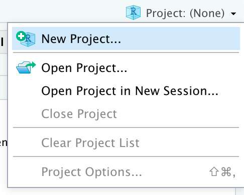
1. You can click the Project drop down menu and choose the “New Project…” option.

1. Alternatively, you can click the “File” menu and choose the “New Project…” option

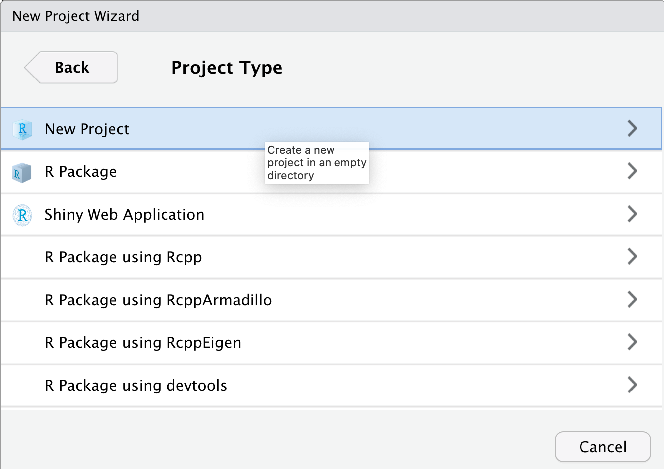
Next the “New Project Wizard” will pop up in RStudio. Since we are starting this project from scratch we will choose the “New Directory” option.

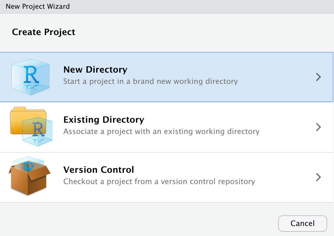
Next the New Project Wizard asks us to chose a project type. We will choose the “New Project” option again.

Finally the New Project Wizard asks us what to name our new project folder, where to put it, and some other options (including if we should make this a git repository).

We will call the folder “example_git_summer_project” and put it on the Desktop. You may need to click “Browse…” to navigate to your Desktop folder. The name is a bit long but will be useful for identifying it when you find it on your desktop or GitHub account later. We also want to be sure the “Create a git repository” option is checked. If you don’t see this option, you may need to check that you have git installed.

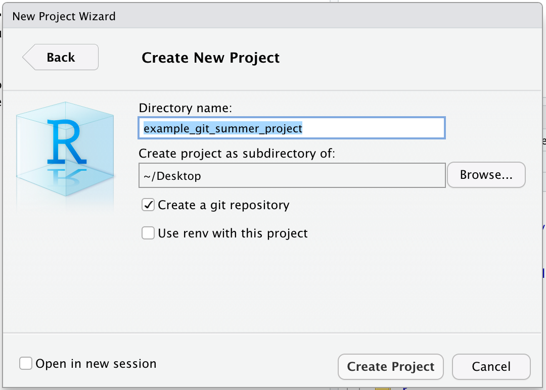
Finally we can click the “Create Project” button.

Find the Project on Your Computer

Use Finder(mac) or File Explorer(windows) to find the project folder on your computer. What files are in the project folder?

Solution

Your folder likely only shows one file in it, example_git_summer_project.Rproj. If you close the project in RStudio (using the project dropdown menu on the upper right-hand side), you can click on this file and it will reopen this project in RStudio.

You probably can’t see it in your file viewr but when we set up the project, we also created a hidden folder where git stores information called .git/. We probably won’t need to interact with this folder directly but it is where git will be storing the history of your files in this project. The folder is hidden by default in most file viewers so we can’t accidently make changes to it. See the following links if you’d like to try to see the hidden .git/ folder

• Windows
• Mac - type Shift + cmd + . to toggle the hidden files showing in finder.

Note: All files that start with . are hidden unless you turn on the option to see them.

Working Locally With Git

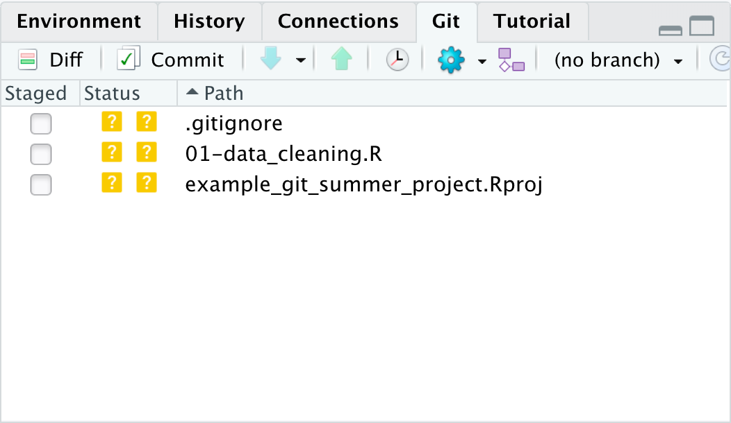
You may now notice that in the Environment Pane (upper right-hand pane of default RStudio), there is now a “Git” tab. This tab is where we can keep track of our files using git. If we click on the tab, we will see it lists a couple of files.

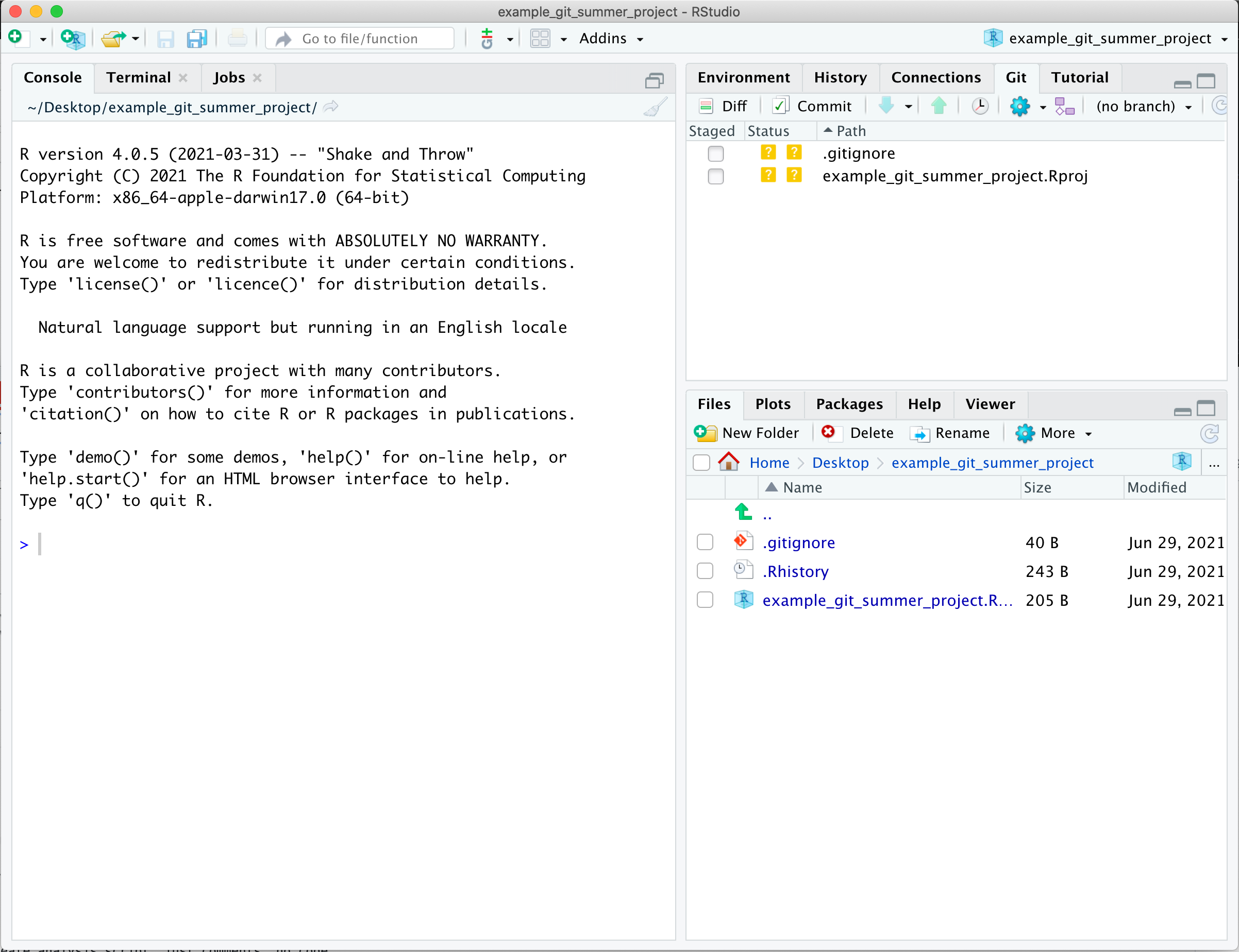
Both the .gitignore and the example_git_summer_project.Rproj file have two ? in the status columns. This means that git recognizes they have changes that are untracked by git.

We will come back to these files later when we talk about the .gitignore file. For now we will ignore them ourselves.

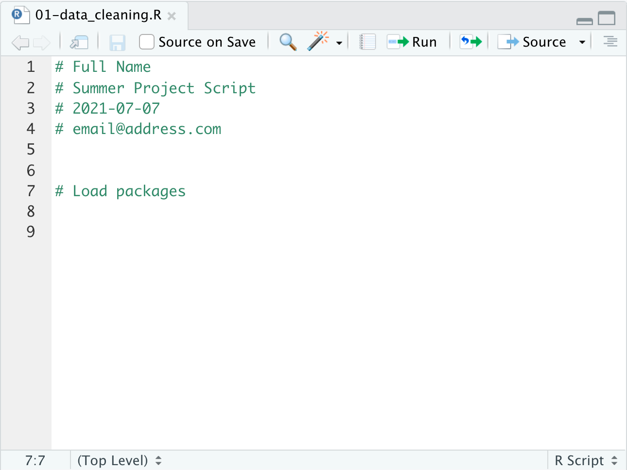
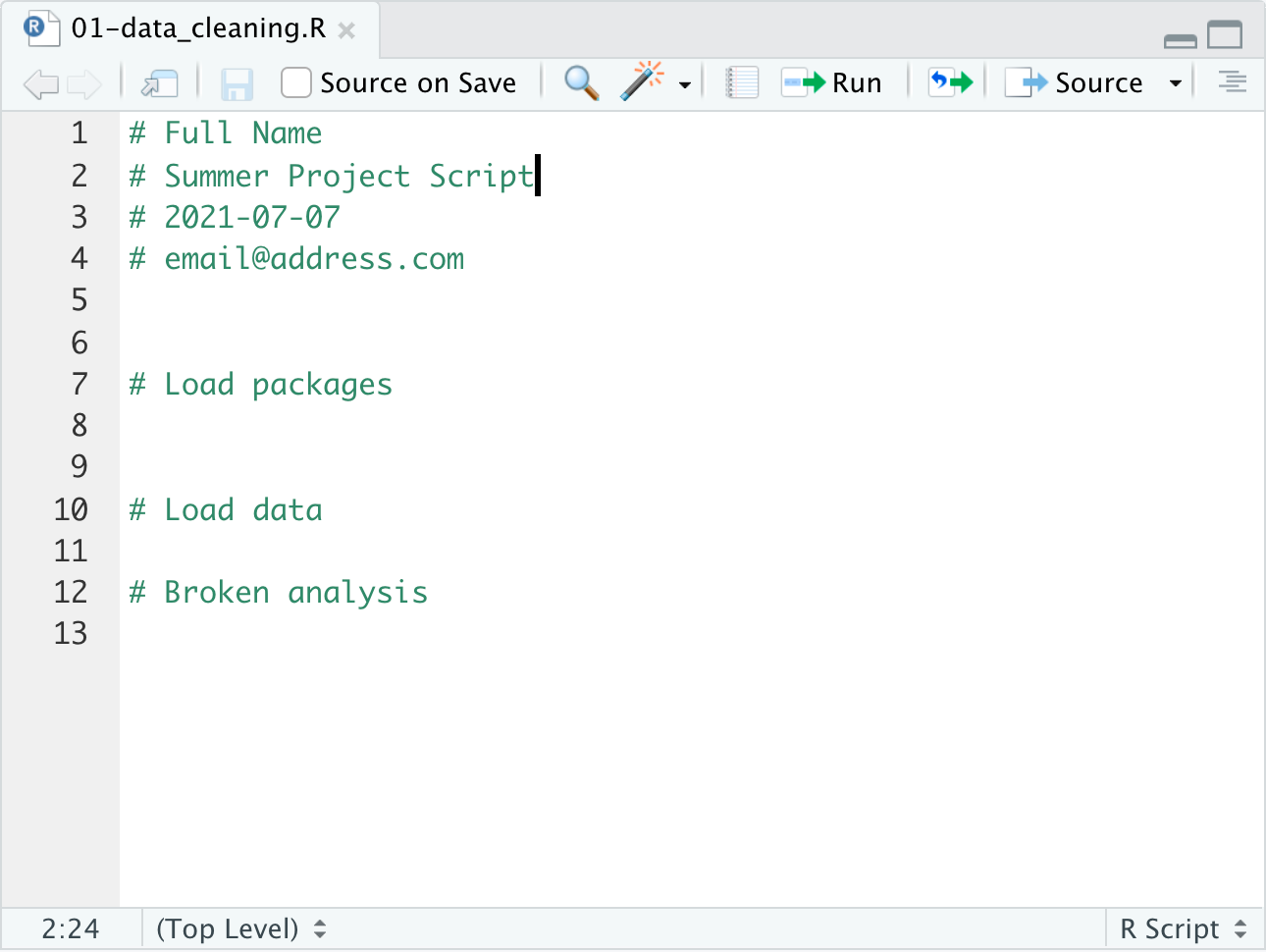
Let’s make a new R script for our summer project analysis. So anyone who finds our script/repo later knows what the script is for and how to contact us, lets add our name, a script desciption, the date, and our email address to the top of the script.

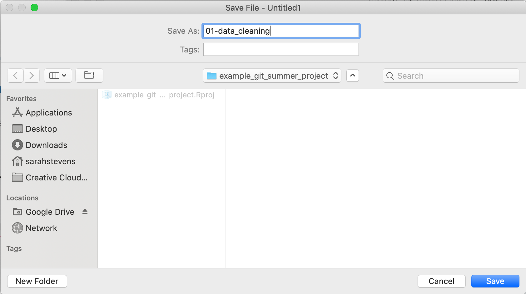
Next we will save the file to a new name. This first script will be our data cleaning script, so let’s call it 01-data_cleaning.R.

Now in the git pane we can see that it shows the new 01-data_cleaning.R script with the two yellow ? around it. This means it recognizes the new file is in the repository and has yet to be tracked.

To tell git we want to keep this version of the 01-data_cleaning.R script, we first click the checkbox in the “Staged” column of the git pane. This adds the file to the stage so git knows to include it in this point of our git history. Once checked the two ?’s turn into an A, for added.

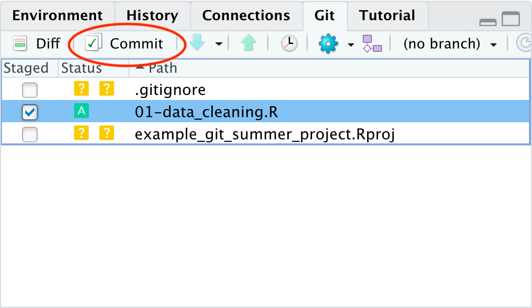
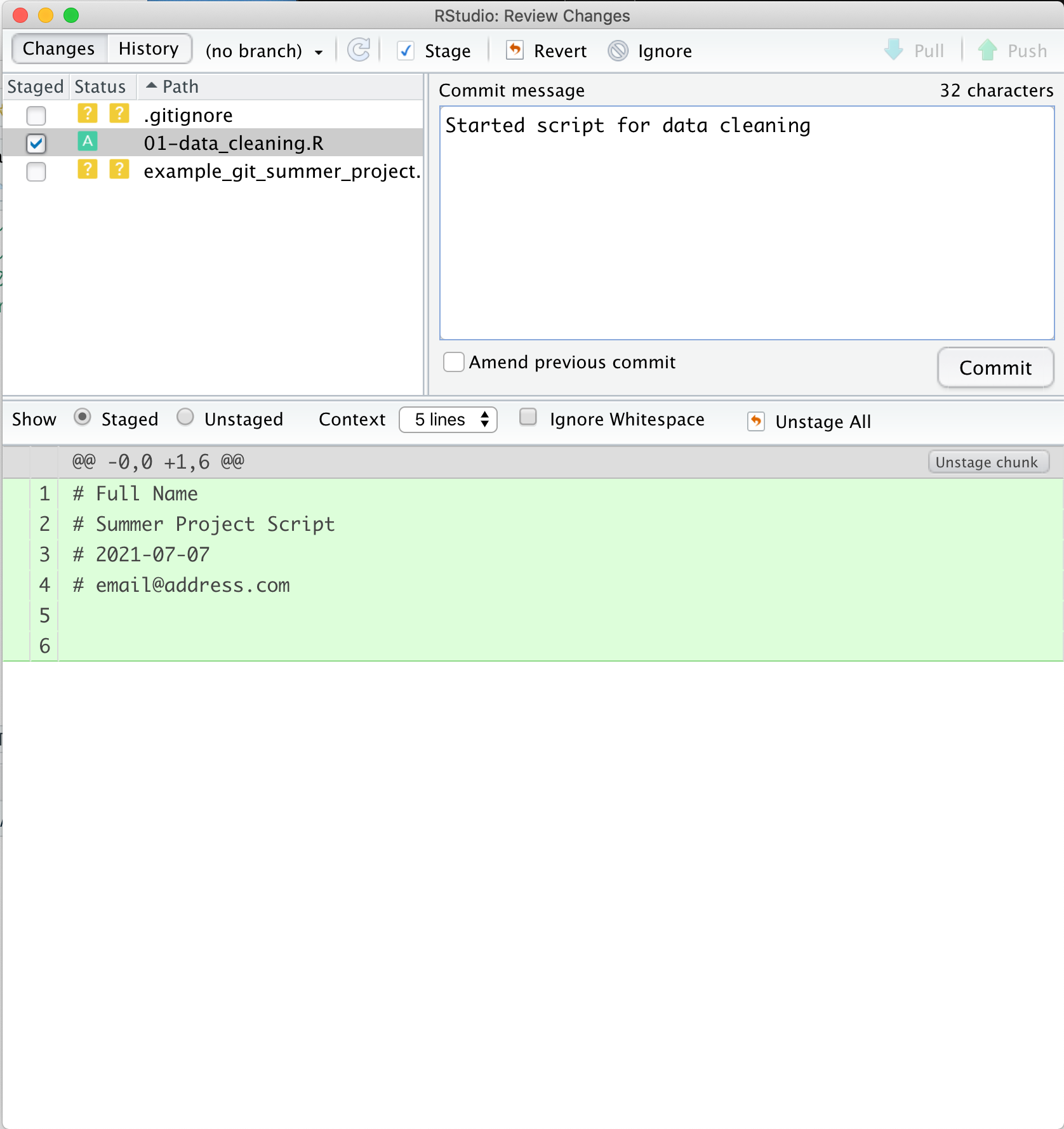
Next we will click the commit button in the git pane (highlighted with a red circle in the image above). When we commit to the repository we add a version of the files that are staged to the git history. Once we click the “Commit” button, a new window pops up to allow for more git interaction. We can see on the left-hand side the same info that we’ve staged the data cleaning script. On the right-hand side we have the opportunity to type a commit message. This message is a note about what was changed in this version of the files committed. We will type Started script for data cleaning as our commit message.

What Makes a Good Commit Message?

The commit message is a great opportunity to leave yourself (or future collaborators) useful information about the history of the repository. While there are other tools to let you see what exactly changed, your commit message can address the motivation for the changes, the “why”. For large changes, it is also a great chance to summarize. Read more about some suggestions for helpful commit messages in this blog post.

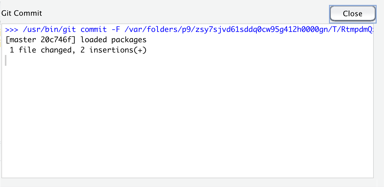
Once we’ve added a commit message, we can click the commit button below the message window. This action actually makes a point in our git history with this version of the file. Once we click this button, we will see another small window pop up with info about the commit we just made. The first line is the command that RStudio ran for us to commit the file using git. The 2nd line gives a lot of information: the branch name (you can have multiple branches for experiments or collaboration, that this is the first commit (root_commit), the first 7 digits of the commit hash - a unique identifer label for each commit, and the commit message we wrote. The 3rd line is a summary of the number of files and lines changed. The last line is info about the file system permissions for the script we created, which we can mostly ignore here.

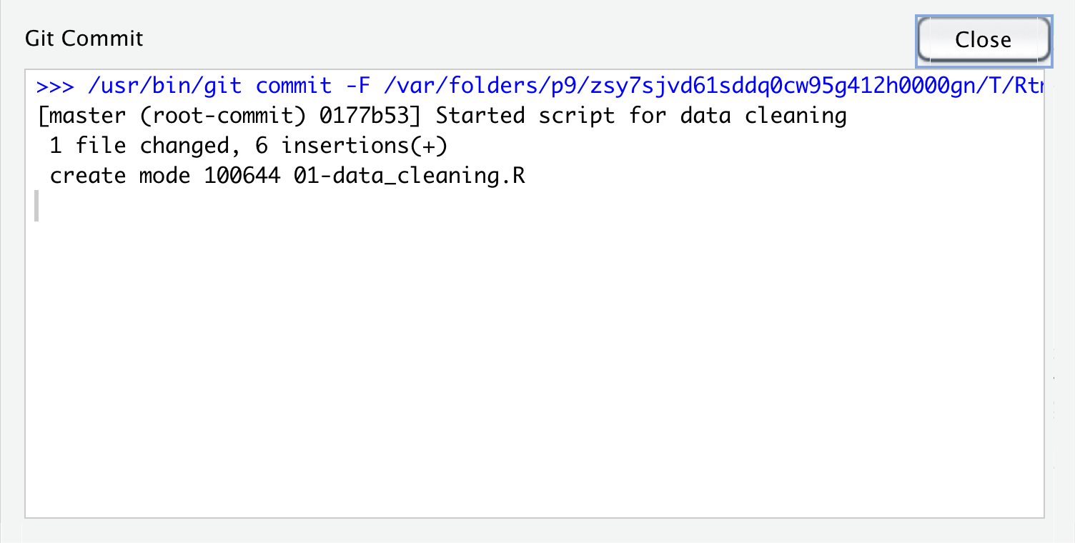
Now that we’ve committed, we can close this pane by clicking the “Close” button. Back in the other RStudio git window, we can see that the data cleaning script is no longer listed in the “changes” window on the upper-left, only the .gitignore and .Rproj files are listed since they have untracked changes. Since all the changes for the data cleaning script are committed to our git repo, it is no longer listed.

Let’s close this window and make more changes to our script. Let’s add a line to load the libraries we want to use. While we are learning git in this lesson, we will write comments instead of actual R code.

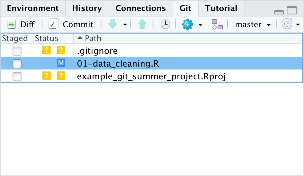
Once we save the new addition to the file, we can see that in the git pane the data cleaning script appears again. This time the status shows as M, which means the file has been modified since the last time it was committed to the git history.

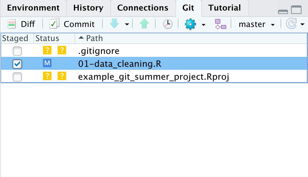
We can follow the same process and add these changes to the stage and and commit this version of the file to our git history. Notice when we check the “Staged” option the M moves from the right side of the status column to the left? This is because those two sides idicate the status in the stage and outside the stage. So the M on the left shows us that we had modified the file but it was unstaged. When we clicked the “Staged” checkbox it moved the M to the left side to indicate the modified file was in the stage. Reminder, the two ? for the other files is because git has not yet tracked them at all, outside or within the stage.

In this commit, notice the bottom of the git window. This section shows the diff, in this case it is showing us the differences between the last time we committed and the new staged version of the file. It highlights in green that we added two new lines. It would show changed lines in yellow and removed lines in red. In addition to the colors, we can use the line numbers to see which lines are changed, added, and removed. The numbers on the left are the old lines and the ones on the right are the new lines. Once we’ve previewed the diff, we can again click the commit button, write a commit message, and click commit.

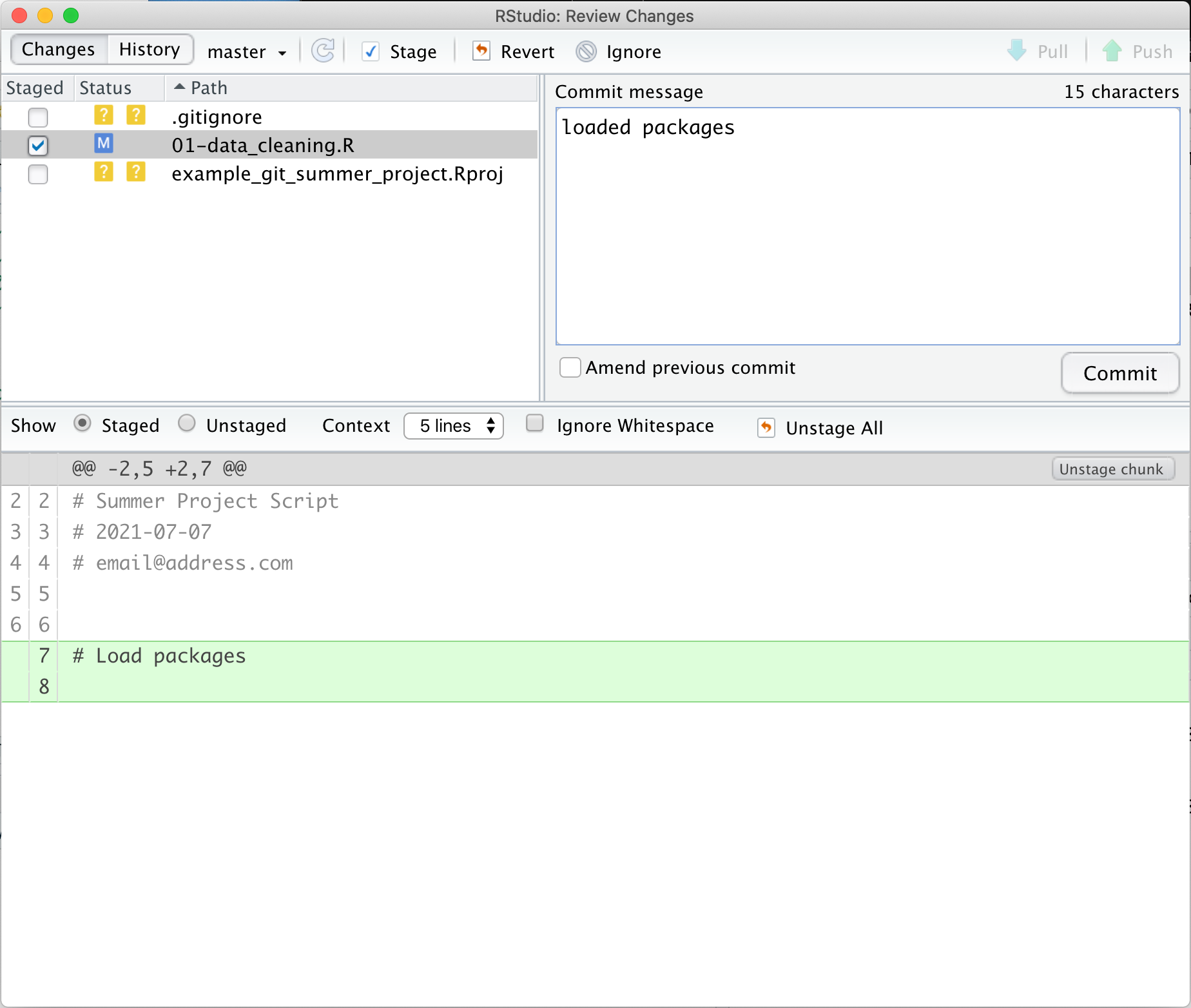
Then we get see the same summary window as before with info about our commit.

Try it yourself!

You will be creating/modifying files, adding, and committing them a lot when using git. Try adding and committing again, this time adding a comment about loading the data.

Exploring your Git History

Now that we’ve made 2-3 commits in our history, let’s take a look at the history so far. Click on the button in the git pane that looks like a clock. Then you will be able to see the history of the repository. Click through and look at the diffs. How can you see the full hash for each commit?

Solution

You can see the full has by clicking on a commit and looking under SHA. SHA is another name for the commit hash, the unique id for each commit. It stand for Secure Hash Algorithm. Often times you can use the shorter version of a hash (as long as it is unique in a repo) to refer to older versions of files.

One of the advantages to using git to version control your project is to get back to an older version of a file. This is possible in a variety of ways from the terminal for other usages. RStudio provides one way to get an old version of a file in a specfic instance, when we’ve not yet commited the new changes.

Lets add a new line to our script # Broken Analysis. This line represents hours spend on a function that doesn’t work and we want to get back to the old version of our script. (In this case we could delete that function but we can pretend there is an old version of the analysis we want to get back to.)

To get back to our old version of the script, we can click the gear/cog icon in the git pane and then click the “Revert…” button. It will then warn us because we have not committed this version so once we revert the only option to get it back would be to code it again. In our case we are sure so we will click “Yes”. Now the script no longer has the broken analysis and is back to the version we last committed. It also is no longer listed as having changes in the git pane.

Other Ways to Get Old Versions

In other situations you might want to keep the broken version in your history by committing first and then getting back an old version. This is possible but would typically be done in the terminal or git bash and would be done with the git checkout or git revert commands.

Note: The git revert action acts differently than the revert we did in RStudio.

Ignoring Files

So far we’ve been ignoring the .gitignore file and the .Rproj file in the git pane. Long term this would get tiresome and we would probably prefer to commit these files to the repository. However there are files we wouldn’t want to commit to the repo. Common files you might want to ignore include:

• data files (since they shouldn’t change much),
• larger files (as these will make your repo get large fast and some hosting services have size limits),
• files that aren’t plain text (you might actually want to commit some of these but they won’t show nice diffs and will take up more space because git will keep a full copy of the file each time it is commited)

Lets create some fake data files and results to ignore in our folder.

• In the Files pane, click “New Folder”, create a new folder called results
• Click the New File button and choose “Text file”
• Save the file as a.dat
• Repeat this process until you have the following files in the project folder:
  • a.dat
  • b.dat
  • c.dat
• Repeat this process and create the following files in the results folder:
  • a.out
  • b.out

Now our git pane will show the new folders and files.

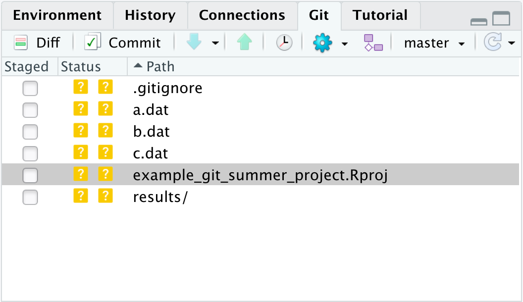
Note that we can only see the one listing for the results folder. Git will try to track any file in our repository, including the directories within subdirectories (though not actually the folder itself). If we try to add the results directory to the stage, it will then let us choose if we want to add all the files or some of the files within that folder. However, we don’t want to add these files the repo, the ones that end in .dat are data files that won’t change and the .out files are the results from an analysis and are rather large (in our imagination).

Instead we can tell git it shouldn’t try to track these files by adding their names to the .gitignore file. Let’s open it and take a look. Double click on the .gitignore file in the Files pane and it will open in the source pane. We can see it actually already has some files included! These files all start with . so we don’t typically see them in our file folders. However, they are important files for R to keep track of the history and other data it uses. RStudio added them to the .gitignore file when we created this project because these are files that are commonly not included in git repositories.

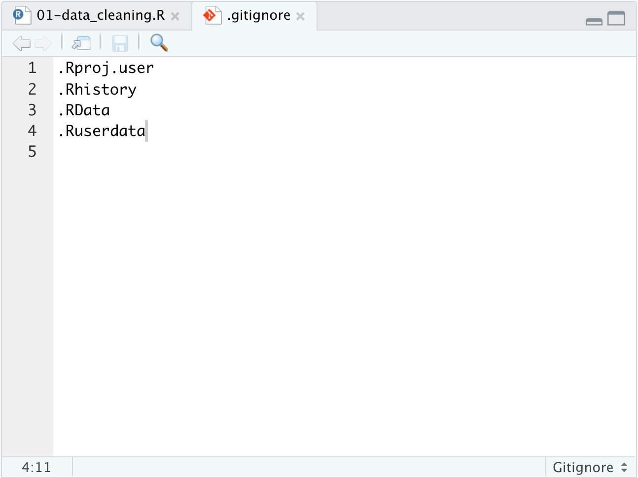
Let’s add a couple lines to the .gitignore file so git will ignore our data and results files. We will add a line using a line that says *.dat to ignore any file that ends in .dat. We will also add a line for the whole results/ folder.

Once you’ve saved, you might notice that nothing changed in the git pane! This is because we need to refresth by clicking the arrow circle button on the right-hand side of the git pane.

Now we can see that the data and results files no longer show up in the git pane.

Adding New Result/Output files

What happens if you add a new d.dat file or results/c.out file? Try it out!

Solution

Those files still aren’t shown in the git pane since they match paterns in the .gitignore file. If later you want to track a single file that matches that pattern, you can add a line to the .gitignore file that has the file name with a ! in front of it to unignore that individual file but ignore the rest of those that match the pattern.

Should We Ignore the .Rproj and .gitignore file?

We could add .gitignore and example_git_summer_proj.Rproj to the gitignore and then we wouldn’t see them listed in the git pane all the time. However these are files that it is good to commit to your repo. Knowing which files you were ignoring on a different machine can be useful if you sync this repo elsewhere later. You will want to have the Rproj setup on the other computer as well.

Add and commit these two files at the same time (with the same commit) to your repo.

Look at History for a Single File

Take a look at your git history, try to figure out how to see only the history for the 01-data_cleaning.R file.

Solution

• Click the History Button in the git pane (looks like a clock)
• Click the “(all commits)” Drop down menu at the top of the commit window
• Choose “Filter by File…”
• Choose 01-data_cleaning.R.
• Now you will not see the commits that don’t include the 01-data_cleaning.R file.

Connecting to GitHub

Creating and Using an SSH Key

So far, we’ve been using Git to version control our files locally. But now we’re going to connect our local repository to a ‘remote’. A ‘remote’ is any git repository that is hosted on the internet, not just on a local computer. In our case, the remote is going to be hosted on GitHub.

Pretty soon, we’re going to create a repo on GitHub and establish a connection between that repo and the local Git repo that we’ve been working with up until this point. But first, we need to create and use some login credentials that will show GitHub that we are who we say we are. This is required so that GitHub repos can only be modified by the people who created or are allowed to access them.

We’re going to use a method of authentication called SSH, which stands for ‘secure shell’ protocol. Basically, SSH is a way for two computers (our local computer and the GitHub server) to communicate, with all information transfer encrypted for security. It operates through public and private ‘keys’, which are strings of numbers and letters.

To connect Git to GitHub, we have to generate a new SSH key. To do that, we’ll follow the instructions in this article to check for an existing SSH key, generate a new key, and save the key (protected by a passphrase).

If you’re on a Windows computer, use Git Bash to run these commands. On a Mac, use the Terminal.

Now that we’ve created a public/private key pair, we’re going to copy the public key and add it to our GitHub account. To do that, we’ll follow the instructions in this article.

Note: This process may seem really complicated and intimidating. Luckily, you only have to do it once, or at least only once per computer you want to set up Git on. You don’t have to set up a new SSH key every time you want to make edits to your project!

Creating a GitHub repository

Now, we’ll go to GitHub and sign in.

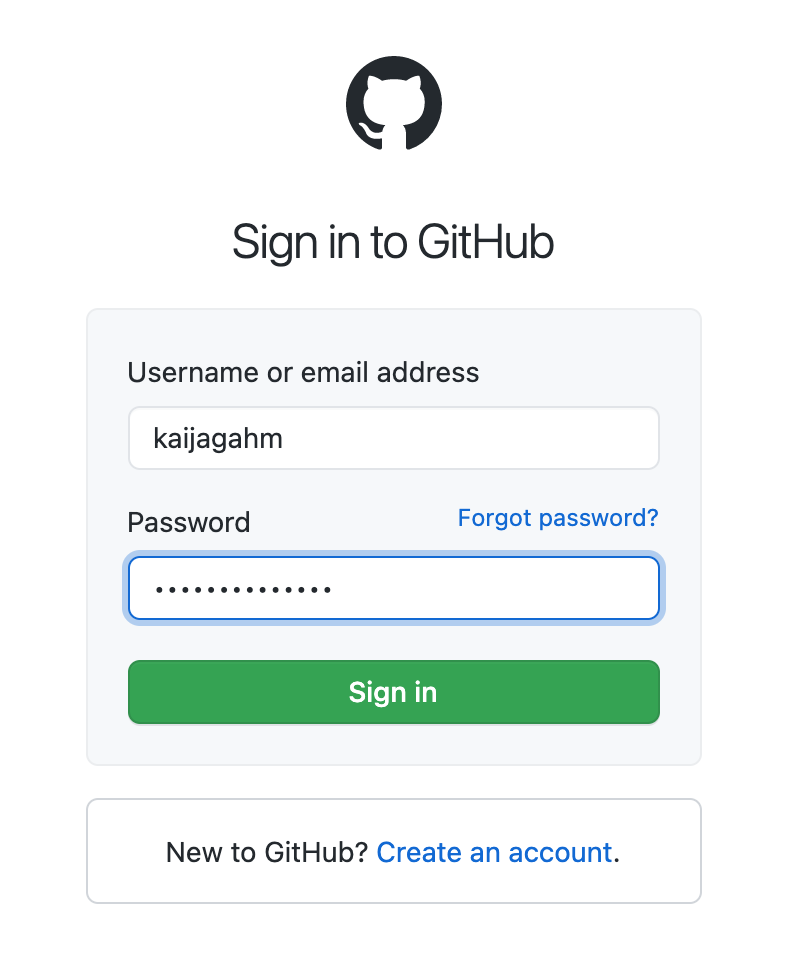
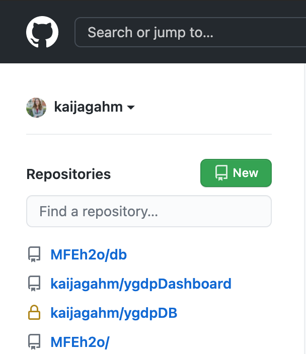
Signing in takes us to a dashboard page, showing all of our activity and listing some of our repositories. On the lefthand side of the page, there’s a toolbar with a heading, under your profile icon, that says Repositories. We’ll click on the green button labeled ‘New’.

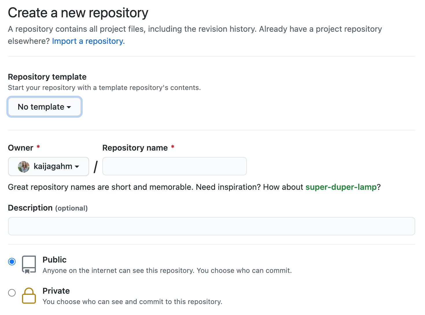
The first thing that we’ll be asked to do is to name our repo. To make things as clear and consistent as possible, we’re going to go ahead and name it the same thing as the local repo that we already created: ‘example_git_summer_project’. If you want, you can briefly describe the repository. Maybe add a note about the context in which you created this repo?

Next, you have the option to choose whether the repository is public or private. If you make it public, anyone on the internet can go to your GitHub account and see this repository. You’ll still be able to manage edit access (so, random people can’t just come in and change your code without your approval). If you keep the repository private, people won’t be able to see it unless you specifically invite them as collaborators.

Public and Private Repositories

Before January 2019, free GitHub accounts didn’t come with private repositories– you had to have a paid account for that. As of 2019, free accounts include unlimited private repositories, each with up to 3 collaborators, according to this announcement. This is an exciting change that’s great for working on private projects!

You should choose whatever repository visibility works for you. If your project includes data or code that you don’t want to share, a private repo might be a good option. But if you keep it public, others can more easily learn from and contribute to your work!

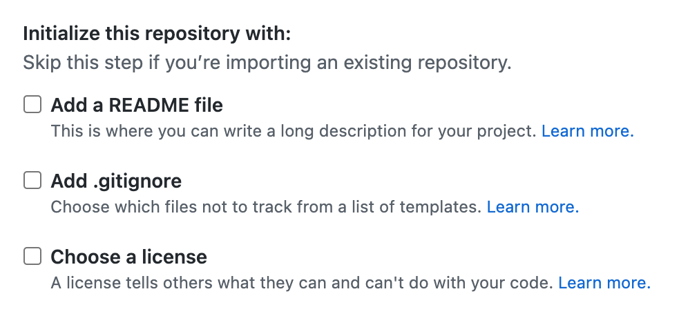
Finally, there are a few more checkboxes, asking you whether you want to add a README, a .gitignore file, or a license. These checkboxes should be un-checked by default. We’re going to leave them that way. Adding a README is a good idea in general and you would probably want to add one eventually if this was a real project, but adding one at this stage can complicate the process of joining the local and remote repos. We already have a .gitignore file in our local repo–that’s the document that we added lines to so that Git wouldn’t track our data and output files. If we create a new one in this remote repo, once again, the process of joining the local and remote repos will get complicated. A license can be a good idea depending on your project–but that’s beyond the scope of this lesson.

Click the green ‘Create Repository’ button, and your repository has been created!

The next page you see will look something like this. In the box labeled Quick setup — if you’ve done this kind of thing before, you’ll notice a toggle where you can choose either HTTPS or SSH, with a box directly to the right that contains a URL. That URL is the web address of the remote repo that you just created. We’re going to use that address to tell our local computer how to connect to the remote. The default is HTTPS, but because we set up authentication with SSH keys, we’re going to choose the SSH option. When you pick that option, you’ll see the URL in the box change slightly.

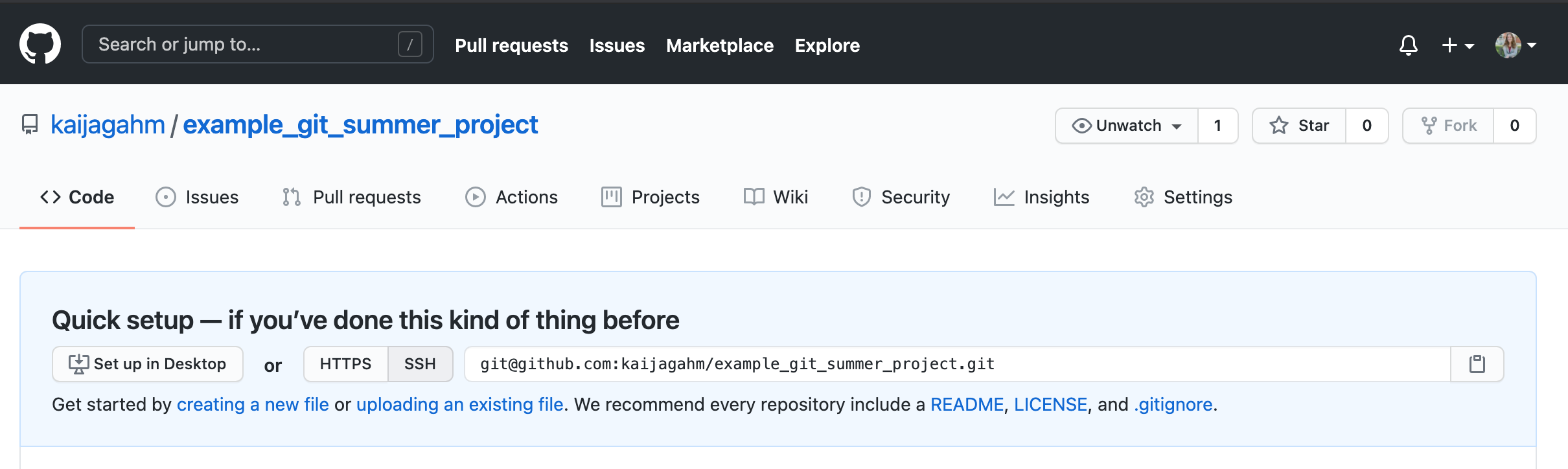
Copy that URL to your clipboard, either by clicking the small clipboard icon at the right, or by highlighting it and copying it manually.

Connecting the Local and Remote Repositories

Now, we’re going to connect our local Git repository to this newly-created ‘remote’ repository. This means that we’ll be able to take changes we make locally and ‘push’ them to the remote repo, where they will be visible and accessible online. As you might imagine, this is very useful for collaborating on a project with other people. But as we’ll see in a little while, it’s also very useful for collaborating with yourself. If you move to a new computer, or if you want to work on the same project from two computers or locations, it will be easy to access your changes from anywhere.

Go back to RStudio, and look at the Git pane. Along the top edge, you should see an icon that looks like two purple boxes and a white square. Click on that icon.

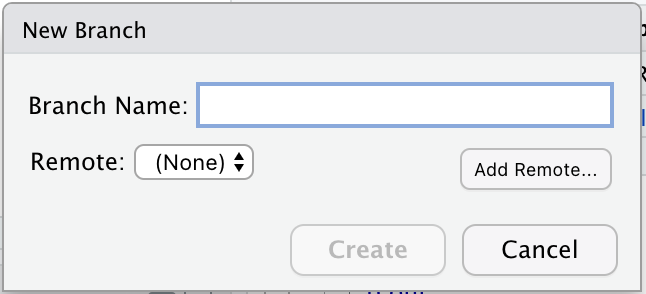
A ‘New Branch’ dialog window will pop up, including a small button that says ‘Add remote’. Click on that button.

Now you will see a new ‘Add remote’ dialog that looks like this.

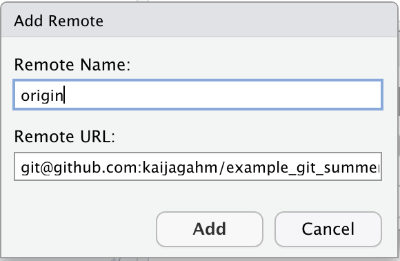
In the ‘Remote URL’ field, paste the SSH URL that you just finished copying from your newly-created GitHub repo. In the ‘Remote Name’ field, type ‘origin’. Now click ‘Add’.

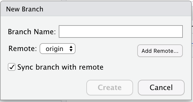
Now you should be back in the ‘New Branch’ window (if you’re not, click on the ‘two purple boxes and a white square’ icon again). We want to make sure that the main branch of the local repo corresponds to the main branch of the remote repo on GitHub. So let’s enter ‘main’ as the Branch Name, and make sure that ‘Sync branch with remote’ is checked. Click ‘create’. This may seem a little weird, since the ‘main’ branch already exists in the local repo by default, but do it anyway.

Because we’re adding a branch that already exists, we’ll see one more dialog, asking if we want to overwrite the existing branch (the ‘main’ branch in the local repo). Click ‘Overwrite’ here (not the default option, ‘Checkout’).

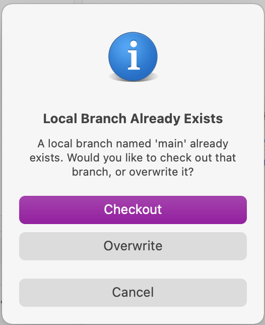
What we’re doing here is making sure that the local and remote branches are all synced up, so that it will go smoothly when we push and pull our changes later on.

Pushing changes

Okay, now we have our local and remote repos connected. Now, we want to push the changes we made locally to the remote, so that they’ll show up on GitHub.

In the top of the Git pane in RStudio, you’ll see two arrows: a blue one pointing down and a green one pointing up.

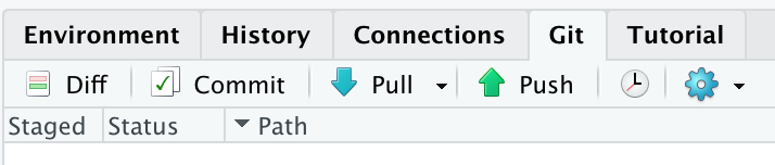
The blue arrow is for ‘pulling’ changes from the remote to your local repo. The green arrow is for ‘pushing’ changes from your local repo to the remote.

Pushing vs. Pulling

If the up and down arrows don’t intuitively match to the concepts of ‘pushing’ and ‘pulling’ for you, it might help to think of your local computer sitting on a table, communicating with the remote repo on the internet, or ‘in the cloud’. If we continue that metaphor, ‘the cloud’ is high up somewhere in the sky, so we pull downward from the cloud to our computer and push upward from our computer to the cloud.

Let’s go ahead and click the green ‘Push’ arrow to push our changes to GitHub.

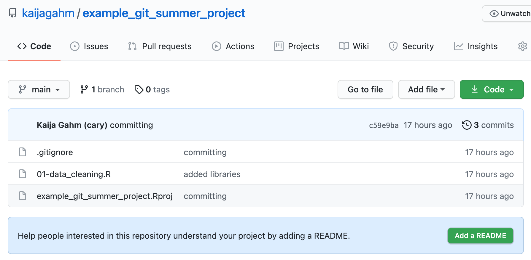
Now, open a browser window and let’s go view our GitHub repo online. If you named your remote repo ‘example_git_summer_project’, then the url will be https://github.com/yourusername/example_git_summer_project.

Opening up the main page of the repo should show us a familiar collection of files. We can see our .gitignore, our .Rproj file, and the ‘01-data_cleaning.r’ script that we created and edited. We can also recognize the commit messages that we entered. The most recent commit message for each file displays immediately to the right of the file name.

Working on a Different Computer

It’s useful to store changes on GitHub for many reasons, but one use case is working on the same project from a different computer. When you were doing field work over the summer, you used a laptop, but once the summer’s over, you might want to work on the same analysis from your desktop computer at home. Since all your analyses are saved on GitHub now, you’ll be able to create a repository on the home computer and connect it to the remote to access those files.

So, let’s pretend you’re now working on your home computer.

The first step to cloning (aka copying) the remote repo from GitHub to your home computer is to create a new R project. We’re going to do the sequence of events a little differently here.

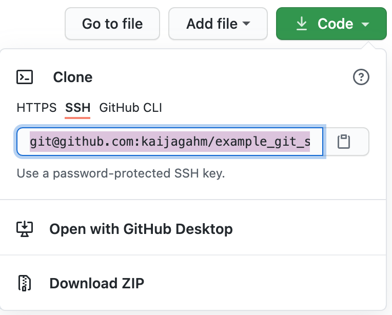
First, go to the main page of your ‘example_git_summer_project’ repository on GitHub. Click the green ‘Code’ download button. A small window will open up with a field that shows the SSH URL (similar to what we saw before). Go ahead and copy that URL to your clipboard, either using the small clipboard icon to its right, or by copying manually.

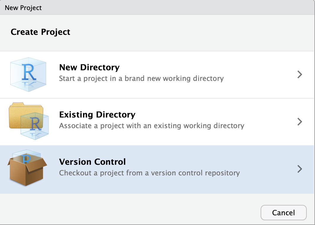
Now, go back to RStudio. Using any of the several methods that we saw before, choose New Project. But then, in the New Project Wizard, instead of choosing ‘New Directory’, pick the ‘Version Control’ option.

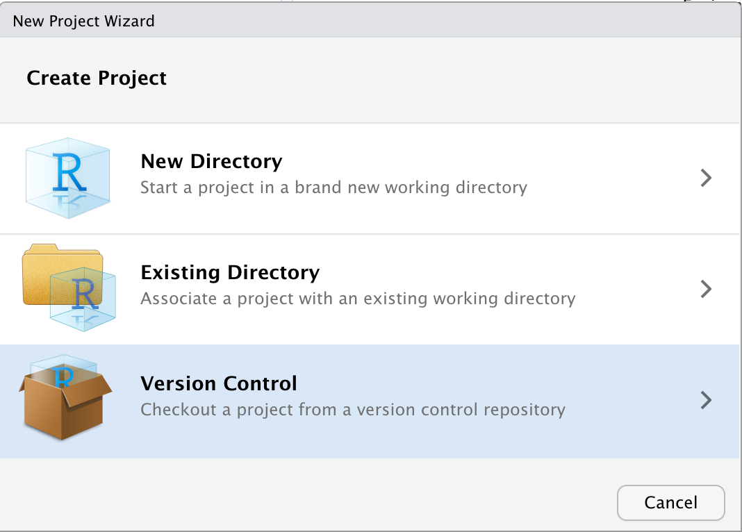
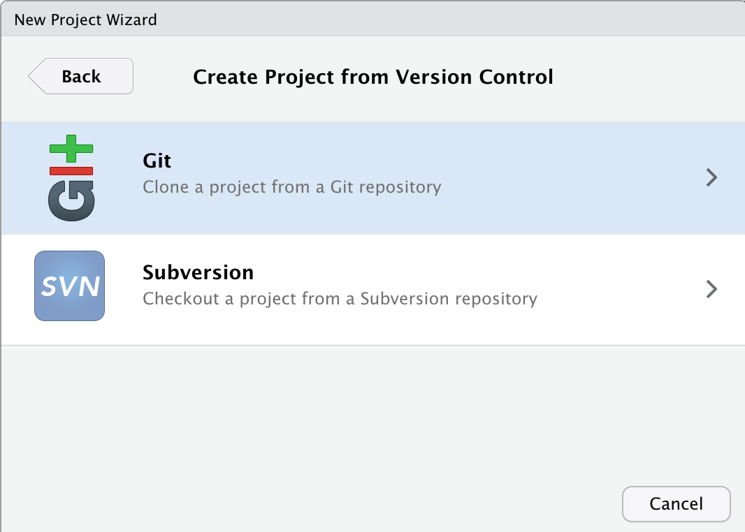
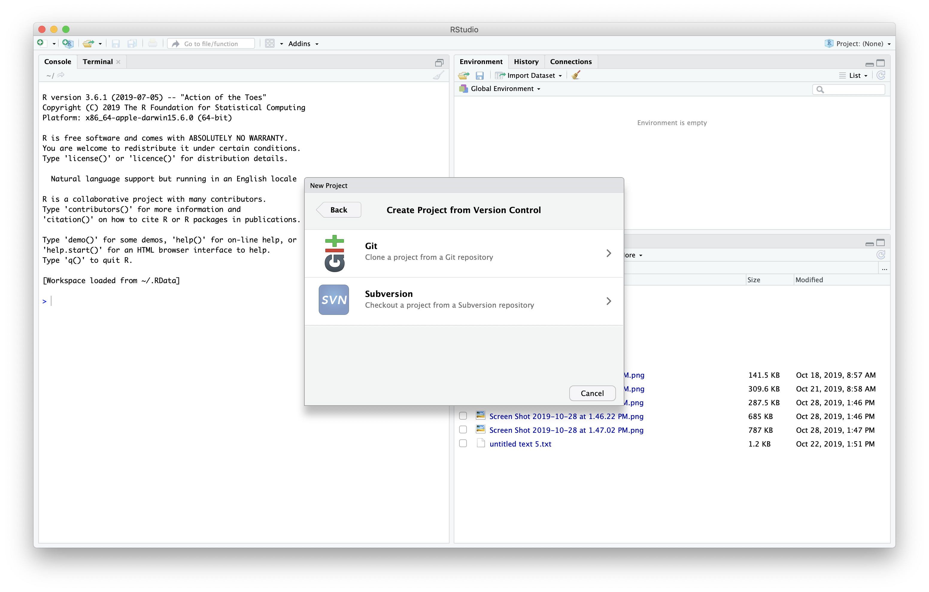
The next window will have you choose which version control software you’re using. Choose ‘Git’. (Subversion is another version control system).

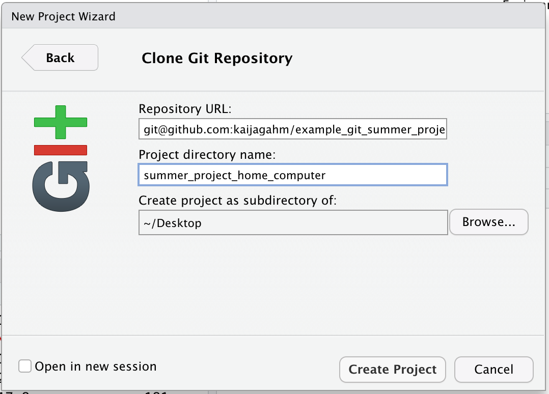
Okay, now we can paste in the URL we copied from GitHub, into the ‘Repository URL’ field. The ‘Project directory name’ field will automatically populate.

Now, here’s the weird part. If we were really working on a new computer, we would be all set here. We could just click ‘Create Project’ and our new project would be created. But since right now we’re working on the same computer as before and just pretending that this is a new, home computer, doing that would create two local repos with the exact same name, which would cause problems. So, let’s change the ‘Project directory name’ to ‘summer_project_home_computer’ or something similar.

Okay, now we can choose ‘Create Project’. RStudio will clone all of the files from the remote repo on GitHub into the newly-created ‘summer_project_home_computer’ local repo, and will automatically open up a new, fresh, RStudio session. As before, you should see a Git tab in the pane next to your History and Environment.

The Files pane should also look familiar now, with our .Rproj, .gitignore, and 01-data_cleaning.R script. But there’s a problem. If you tried to run your analyses right now, on this new computer, you wouldn’t be able to. Why?

Setting Up a Project on a New Computer

What other steps might you need to take to get this project ready to run, so you could seamlessly replicate the analyses you ran on your field computer?

Solution

Because we added our data and output files to the .gitignore, Git doesn’t track them. That means they don’t show up on the remote GitHub repo, which in turn means that when we clone/download the data and code from the remote to our home computer, the data and output files don’t come along. So, if you wanted to re-run your analyses and have everything work, you would have to manually transfer your data files from the other computer to this one. Then, you could re-create those output files by running the R scripts that read in the raw data.

So, this is one of the weaknesses of relying on version control: you still need a system for managing your data. Let’s talk about possible ways to store and manage data, depending on whether it needs to be private or not. What are some strategies or workflows you’ve used in the past or might use in the future for storing data in tandem with version-controlled workflows?

Okay, so now we have our project set up on the home computer. Let’s go ahead and do a little work! Make a change to the 01-data_cleaning.R script, and commit it, writing a commit message.

{What questions do you have about making and committing a change? Do you remember how we did it before?}

Now, let’s pretend you switched computers back to the laptop you used in the field. So we want to switch back to our ‘example_git_summer_project’ local repo (again, pretending that we are actually switching computers).

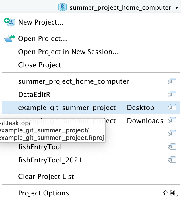
There are a couple ways to do this. 1) You can navigate to the ‘example_git_summer_project’ directory wherever you stored it on your computer, using Finder/File Explorer. 2) At the top of your ‘summer_project_home_computer’ session of RStudio, there’s an R Project icon that shows the name of the current project. Clicking that brings up a dropdown menu that we’ve seen before, with the option to create a new project or select one of the recent projects you’ve been working on.

Either way, open up that project. Now open the ‘01-data_cleaning.R’ script. The change you just made on your home computer isn’t there. Why? How can we fix this?

Syncing Changes Between Local Repos

Why doesn’t the change you made on your home computer show up in the repository on your laptop? How can we get it to show up there?

Solution

We made a change to the local copy of the script saved on the home computer, but we didn’t Push that change, so it won’t show up on GitHub. If we go ahead and click ‘Push’ in the home computer repo, now the change will show up on GitHub (you can navigate to the repository page and refresh it to be sure). But if you navigate back to the ‘summer_project_home_computer’ project, that change still doesn’t show up! That’s because we also need to Pull the change down from GitHub to this other local repository. So, syncing the repositories is a two step process: After making local changes, Push them to GitHub so they can be accessed, and then in the new local repo, Pull down from GitHub to make sure your copy of the repo is up to date before starting to work. It’s always a good idea to Pull changes before you begin to work in a remote repo, especially if you’re collaborating with other people who may have made changes while you weren’t working, but even if it’s just you and you have multiple clones of the same repo in different locations.

This process of pushing and pulling to keep things up to date is very important. In the next section, we’re going to explore the conflicts that can come up if you forget to push/pull, and how to deal with them.

Dealing with merge conflicts

So, what if we forget to push and pull? Let’s act out this scenario so we can see what happens.

First, open up the ‘summer_project_home_computer’ project (i.e. open the project ‘on your home computer’). Make a change to the 01-data_cleaning.R script, on line 3 (you can just add a comment). Commit your change, and push it.

Great. Now, let’s imagine that you’re working on the project temporarily from your field laptop again, and you want to do some coding. Open up ‘example_github_summer_project’ (i.e. open the project ‘on the field laptop’). Don’t pull.

You want to add a data cleaning step to line 3. You’re a little confused, because you’re pretty sure you already added that step the other day, but you don’t see it here. “Huh”, you think. “That’s funny. Oh well, I guess I must have forgotten to save my work!” It’s no big deal, since you remember what you wrote. Go ahead and make your change (a comment, for our purposes) on line 3 of the script.

Commit your changes and push. Uh oh! The push gets rejected. You get a big scary error message.

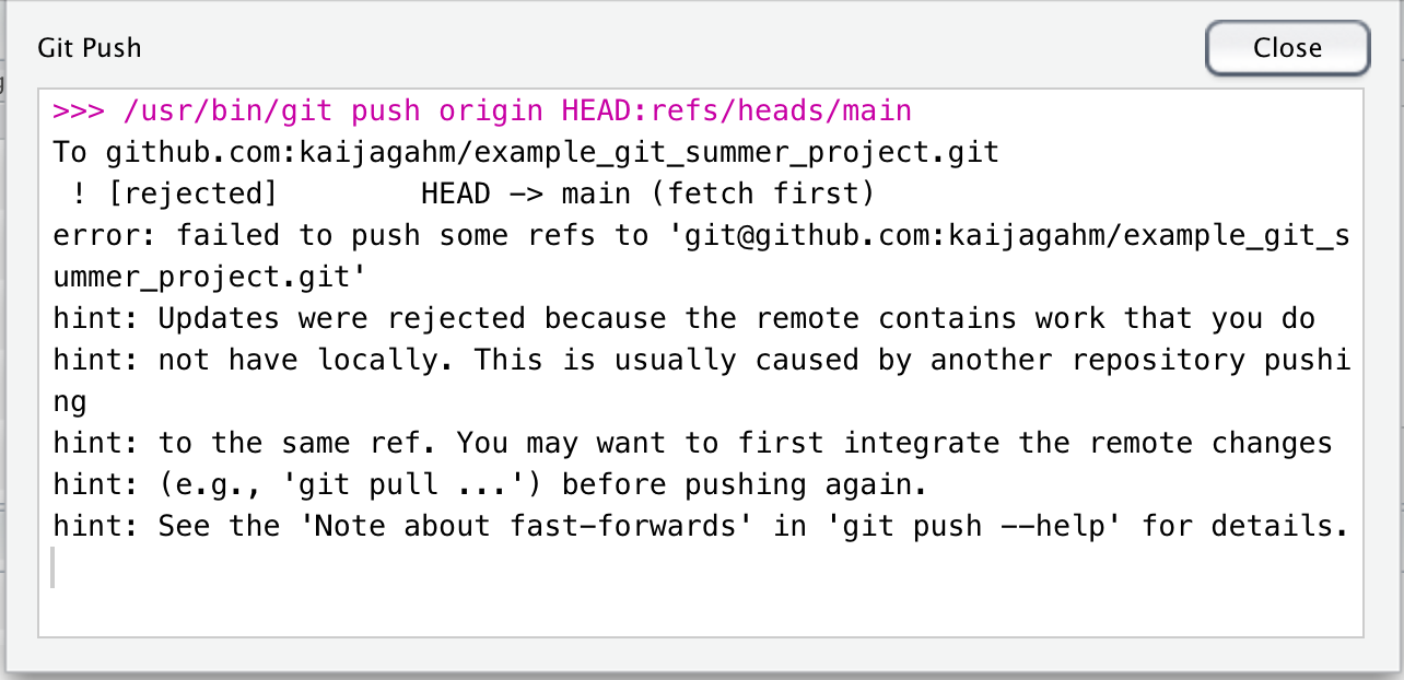
But if we read the error message, it’s actually pretty informative. It says “Updates were rejected because the remote contains work that you do not have locally. This is usually caused by another repository pushing t the same ref. You may want to first integrate the remote changes (e.g., ‘git pull …’) before pushing again.”

So, this tells us what our mistake was: we should have pulled changes from the remote before pushing new changes.

We have created a merge conflict. Merge conflicts happen when there are two changes made to the same line of the same file, and Git doesn’t know which one to keep. If we look back at the staged/status window, we see a new icon, a U. The diff window shows that both the old change and the new change to this file are present, and we also see some lines of = signs and < > signs.

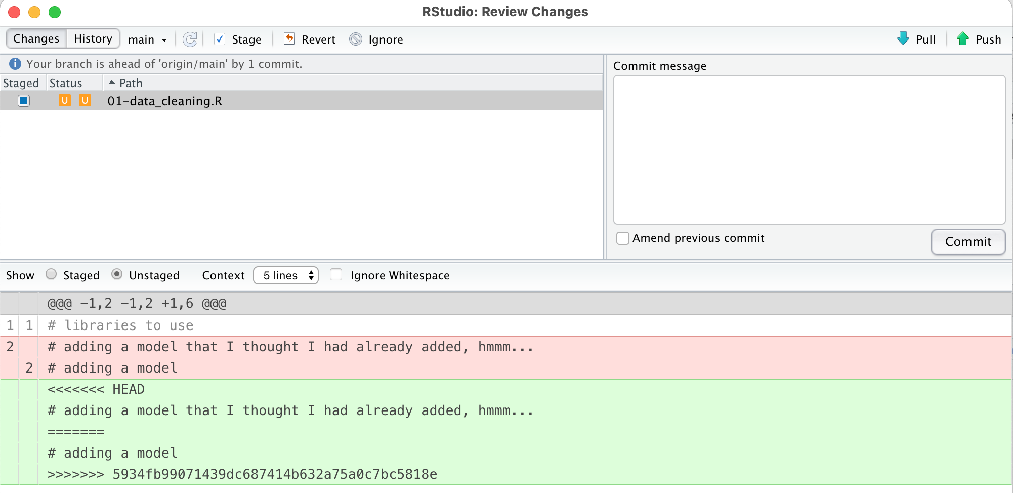
So, how do we fix this?

Open up the file and decide which of the changes you want to keep. Manually delete the «« and ===== and »» lines, as well as deleting the change that you want to get rid of.

Now, stage and commit this fix. Your commit message could be something like ‘resolving merge conflict’.

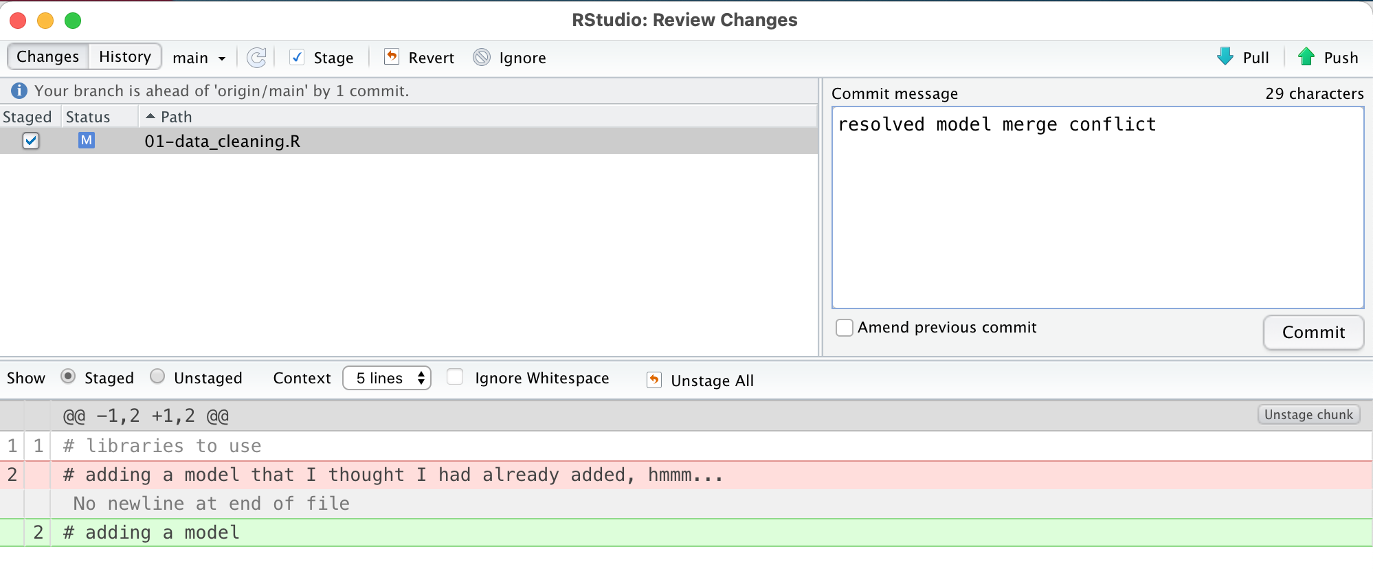
And now push your changes. Ta-da! The repository is all fixed.

Committing and Pushing

How often, or after what activities, might you want to commit and/or push? What are the tradeoffs?

Key Points

• FIXME

R version control for collaboration

Overview

Teaching: 0 min
Exercises: 0 min

Questions

• Key question (FIXME)

Objectives

• First learning objective. (FIXME)

In the last lesson, we learned how to collaborate with someone by giving them collaborator access to our repository. In this lesson, we will learn how to suggest changes to a repository we don’t own.

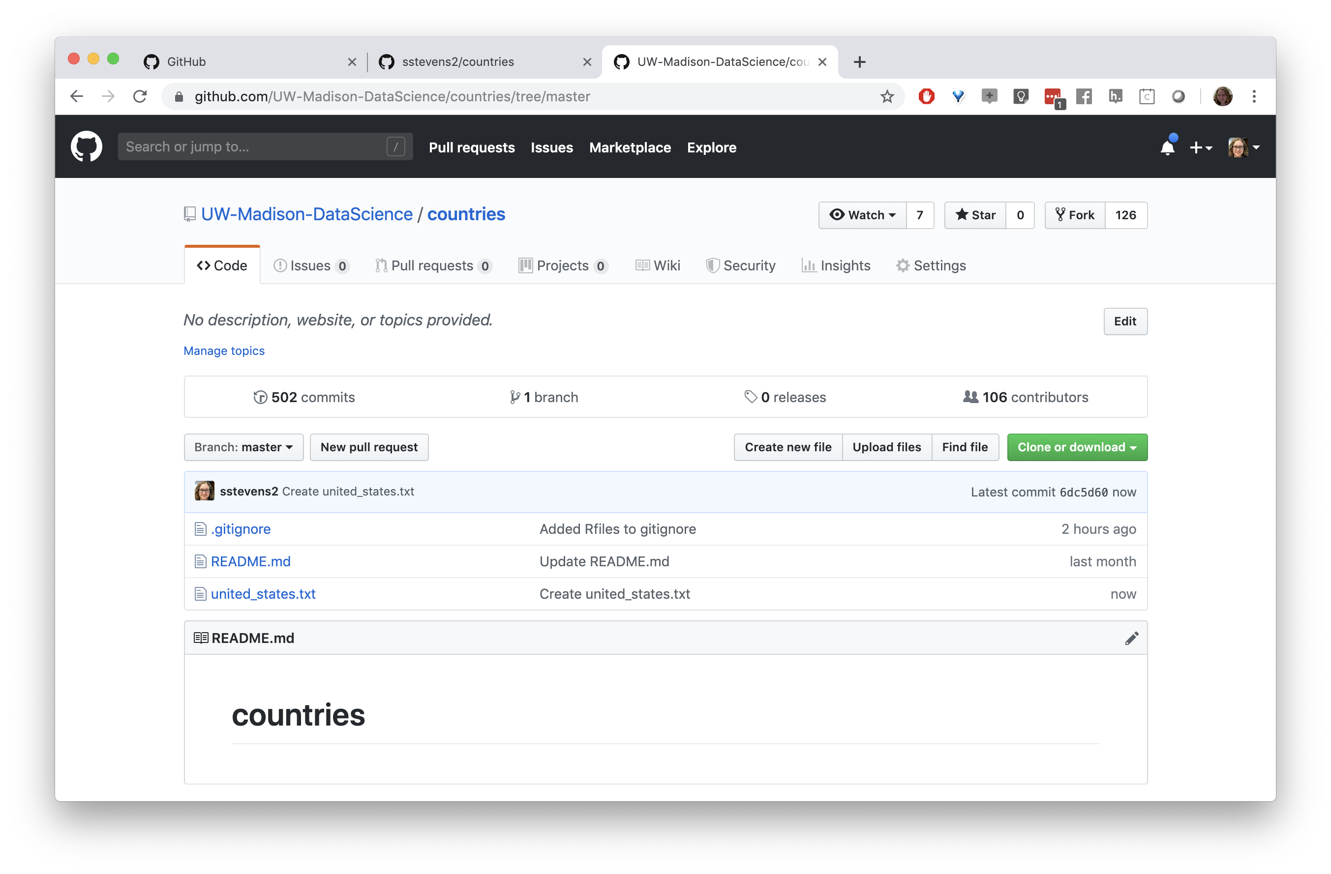
First we will navigate to the github repository we want to make a suggestion to. In this case we will be adding a country to a group repository.

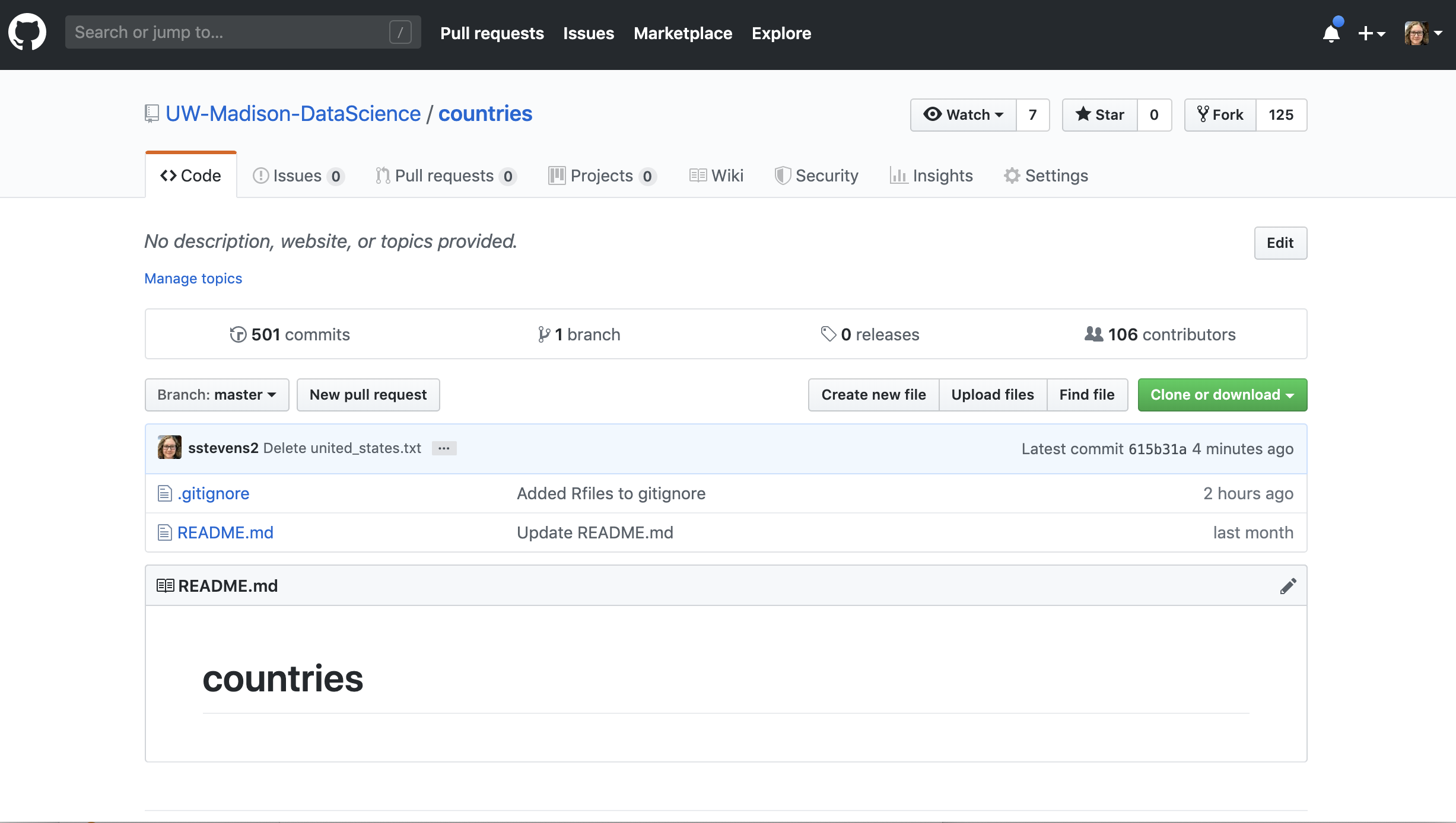
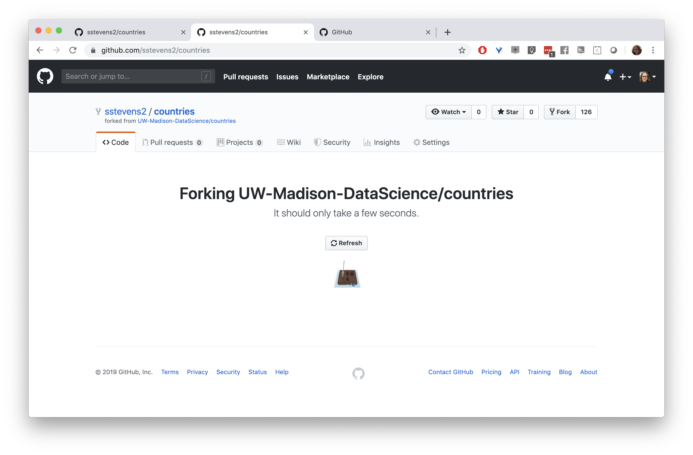
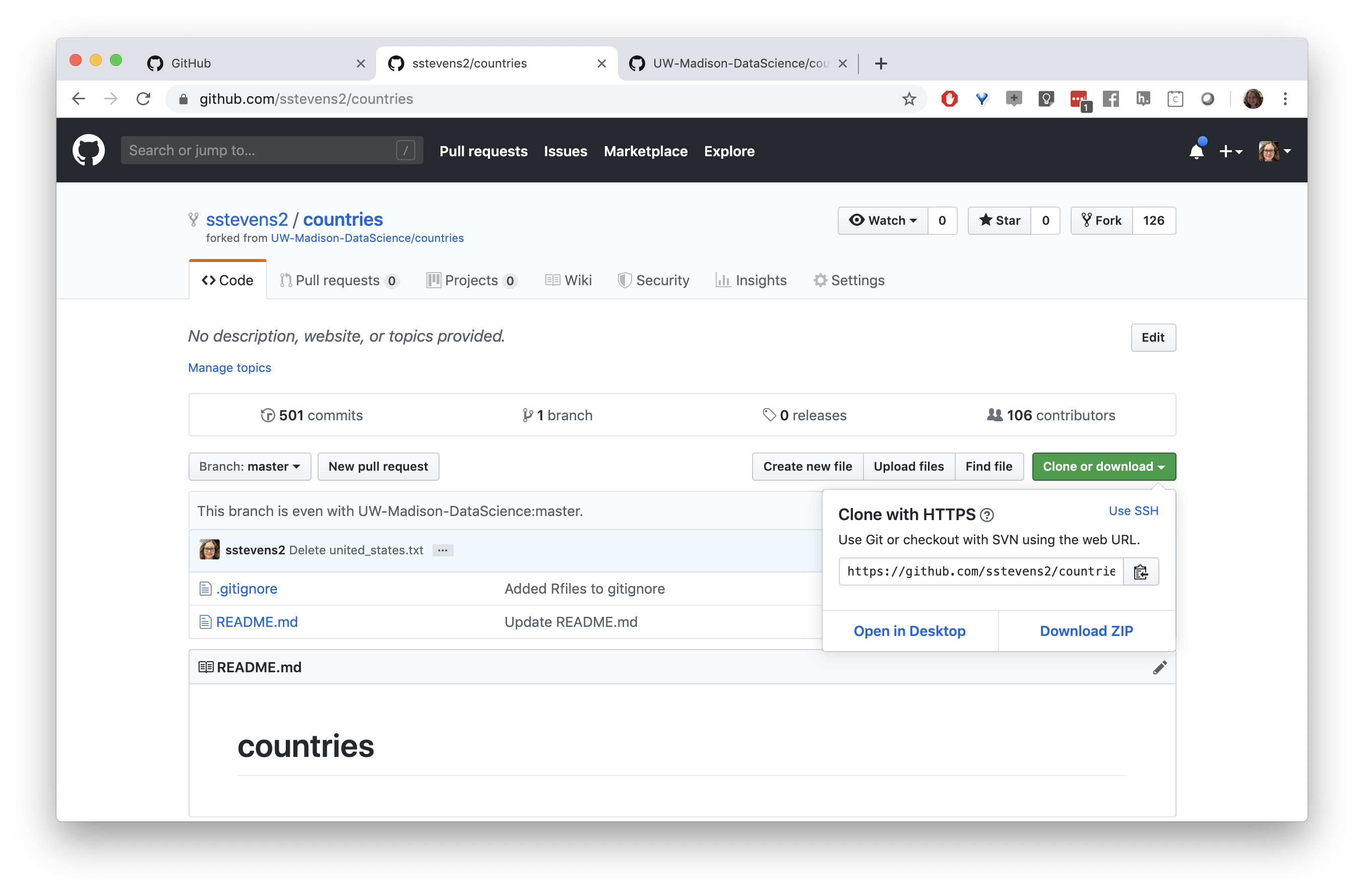
The first ting we need to do is “fork” the repository. This means we will make a copy of this repo that we have access to modify. We will click the “Fork” button in the upper right hand of Github.

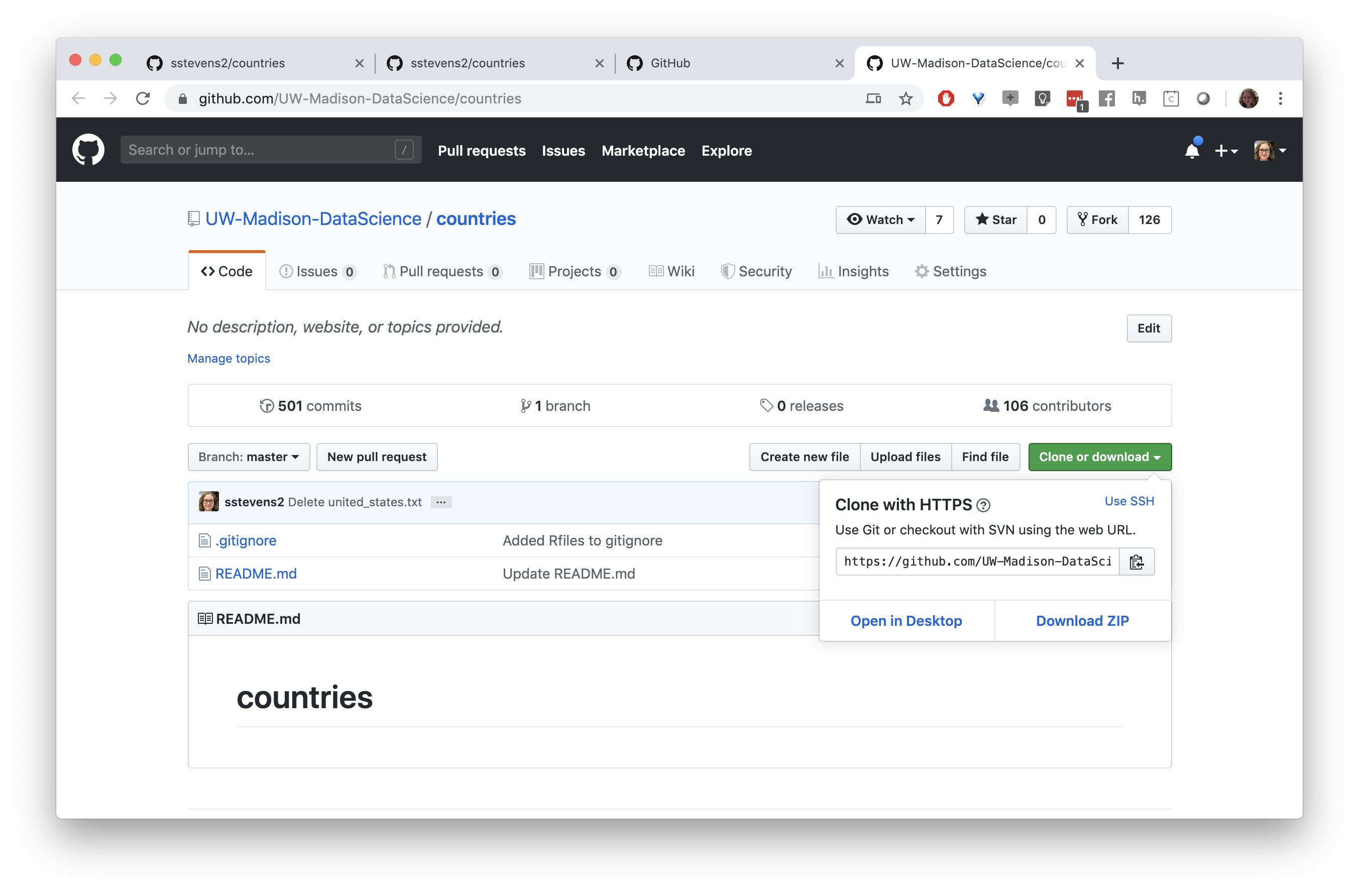
Next we need to get a copy of this repository on our local machine (and in Rstudio). We need to go back to the original repository, which is linked under the repo name. We can clone the repository by copying the link under the “Clone or download button”

In R studio we will start a new project and choose the “Version Control” option.

Next we will tell it to expect a git repository.

Finally we will paste the URL, give the project a name (or leave blank to keep the repo name), and tell it which folder to put the project in. This will copy down the repository to our local computer.

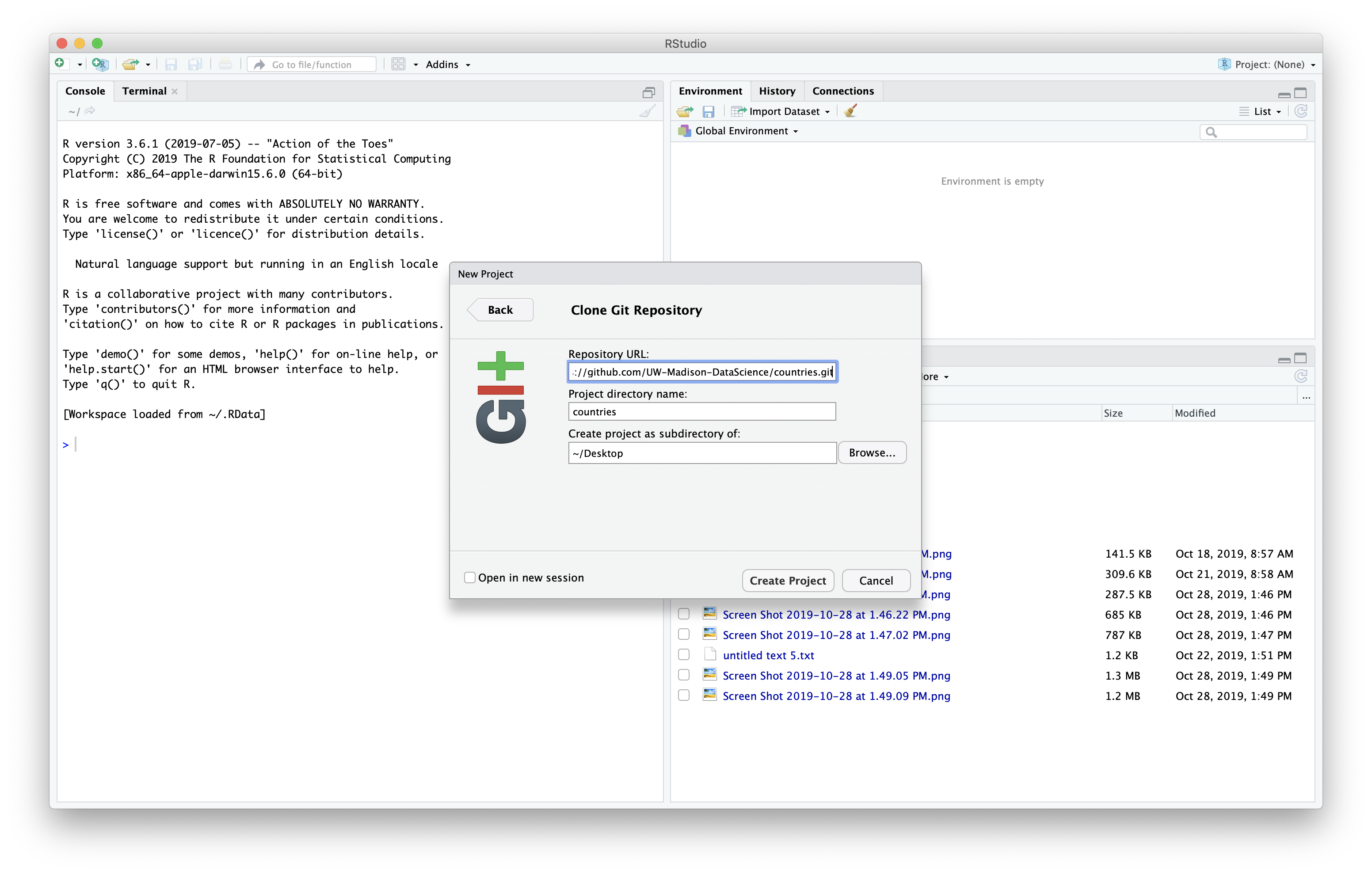
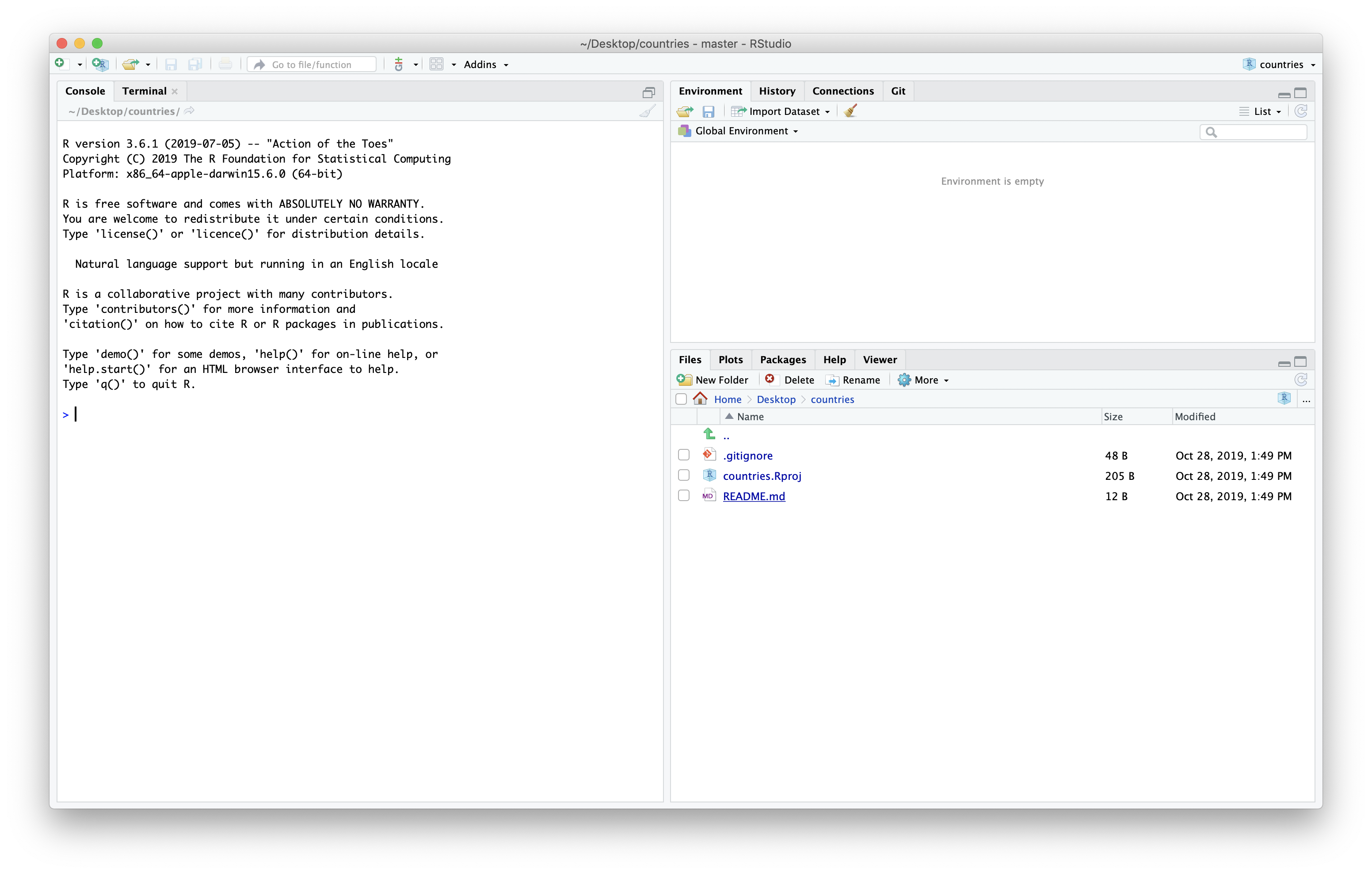
Now we have the repository as a project in Rstudio. This repo has been setup with a .gitignore and README.md file.

Now our repository a connection to the main version of this repository but we also need it to have a connection to our fork of the repository. First we click the “New Branch” button in the git tab.

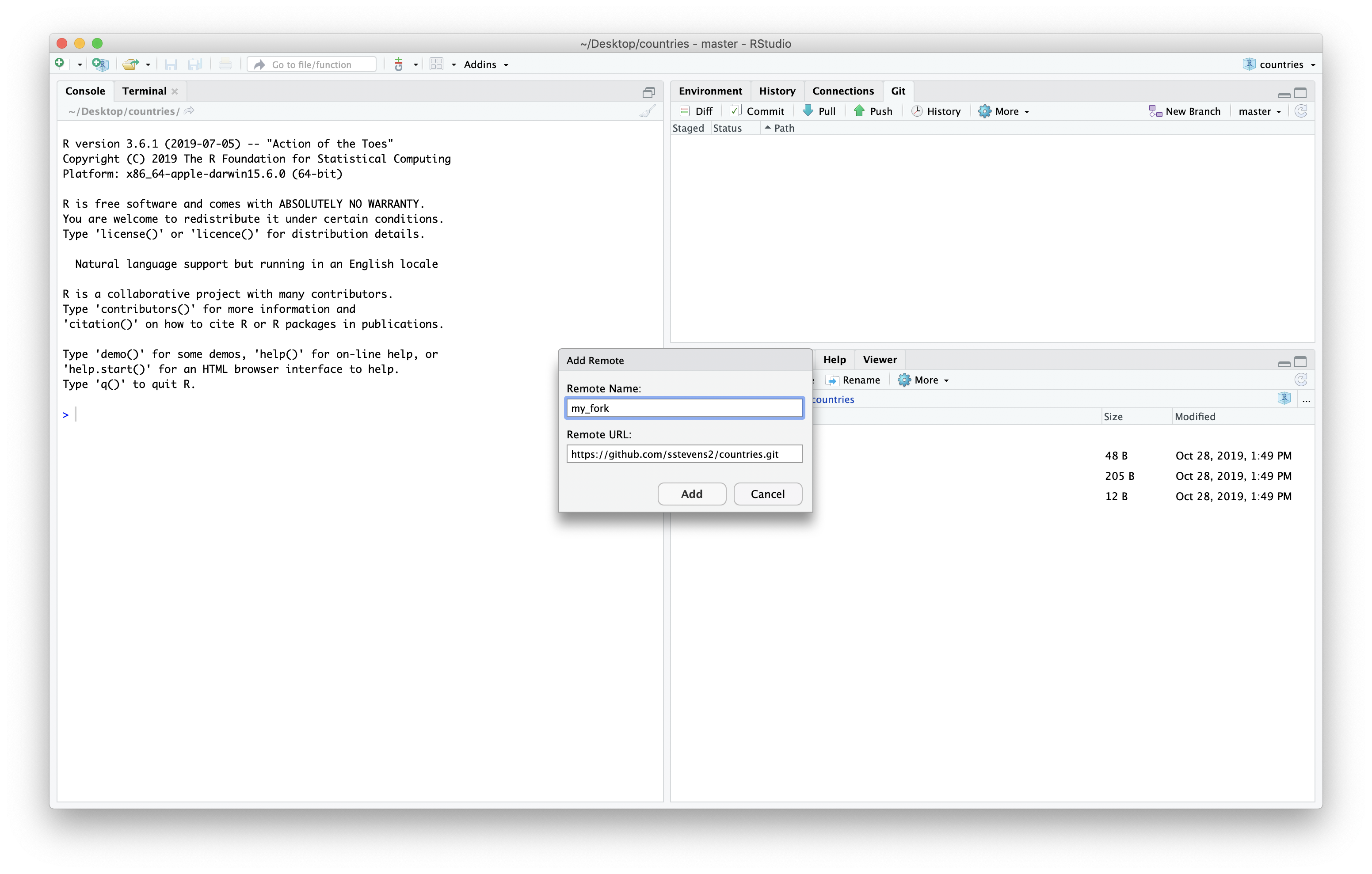
We can then click the “Add Remote…” button to add our fork as a remote.

The ‘origin’ remote is the one we cloned the repo from originally, in this case the main repository. We will need to switch back to our fork and copy the URL from the “Clone and Download” button again.

Let’s call this remote “my_fork”, then paste the URL to our fork of the repo, and press the “Add” button.

Before we make our changes we want to be sure we have the latest version of the main repository. It turns out, since we cloned it one of our colleagues added a file to the repository.

We can use the git tab to pull down the latest changes.

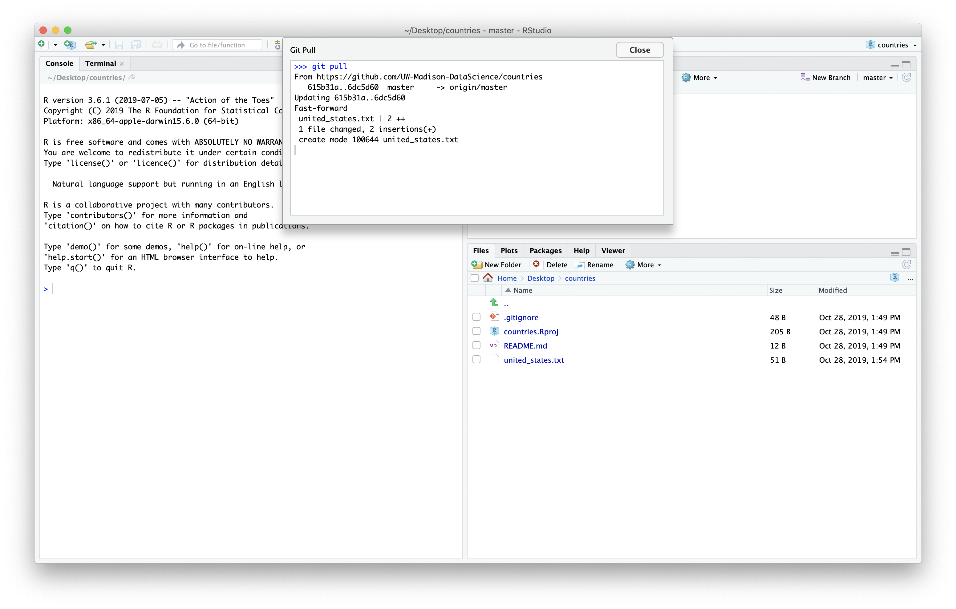
We can see the new file in the file panel of Rstudio.

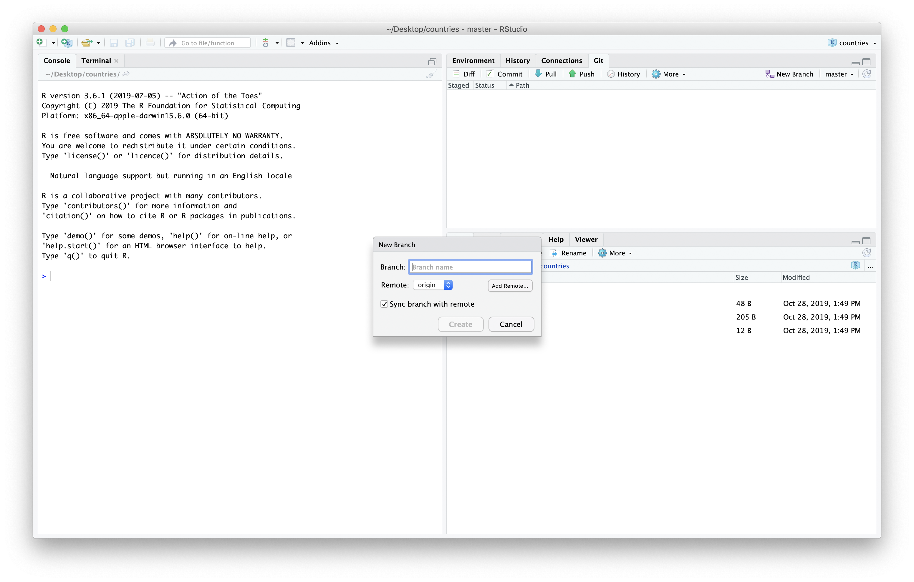
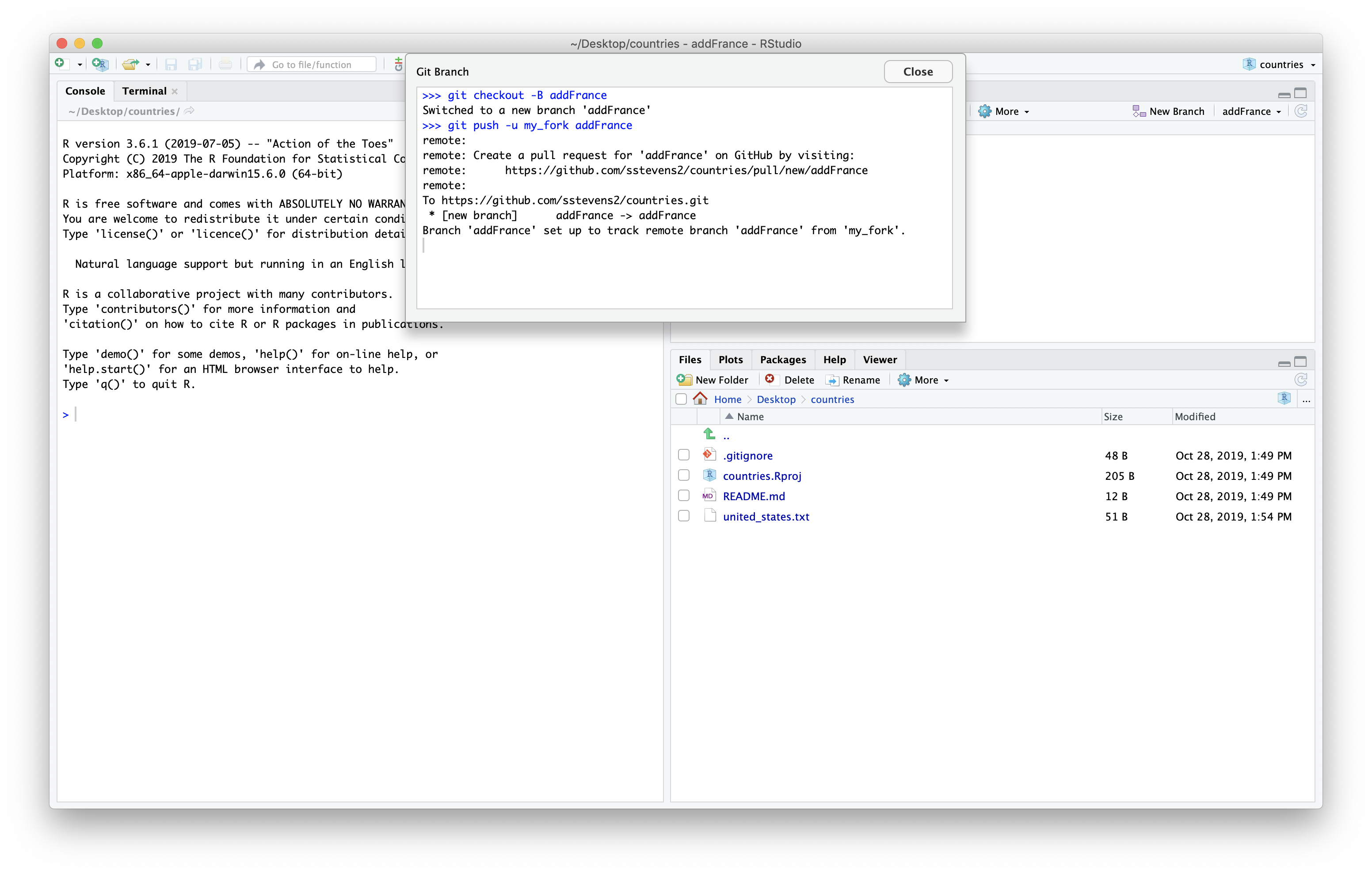
Before we make the changes, let’s make a new branch to work in. This way we can keep the master branch in line with the main repo. We can make a new branch using the “New Branch” button in Rstudio.

We then will give our branch a new name. I’ll be add the country France to the repository so I’ll all my branch “AddFrance”. Be sure choose the remote “my_fork” since that is where we will want to push the changes to when we are done. Then we can click “Create”.

Next we can use Rstudio as a text editor and look at the united states file.

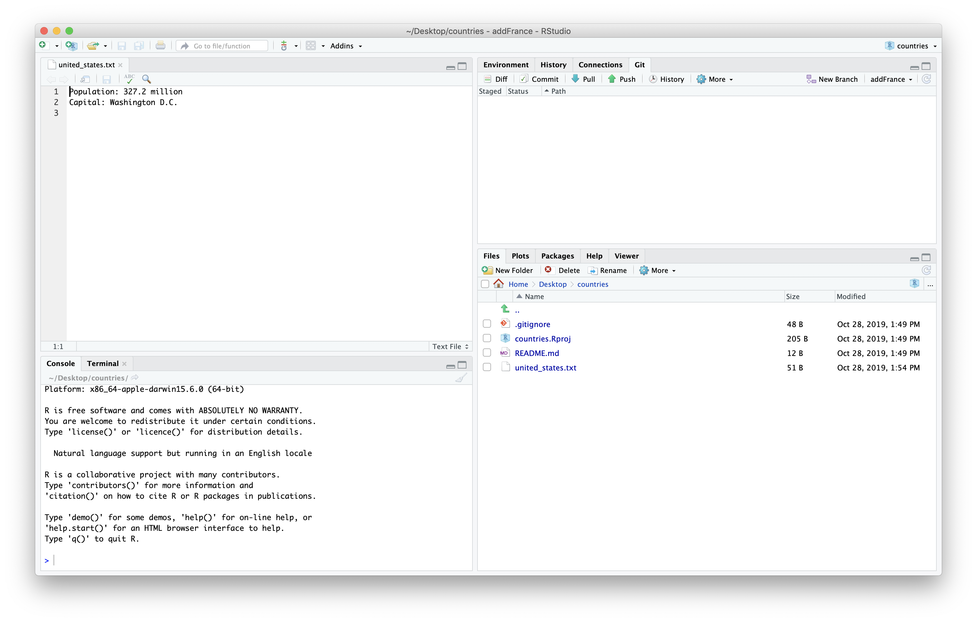
We can then make a new country file and update the information. You may need to look up the information for you country in the web browser.

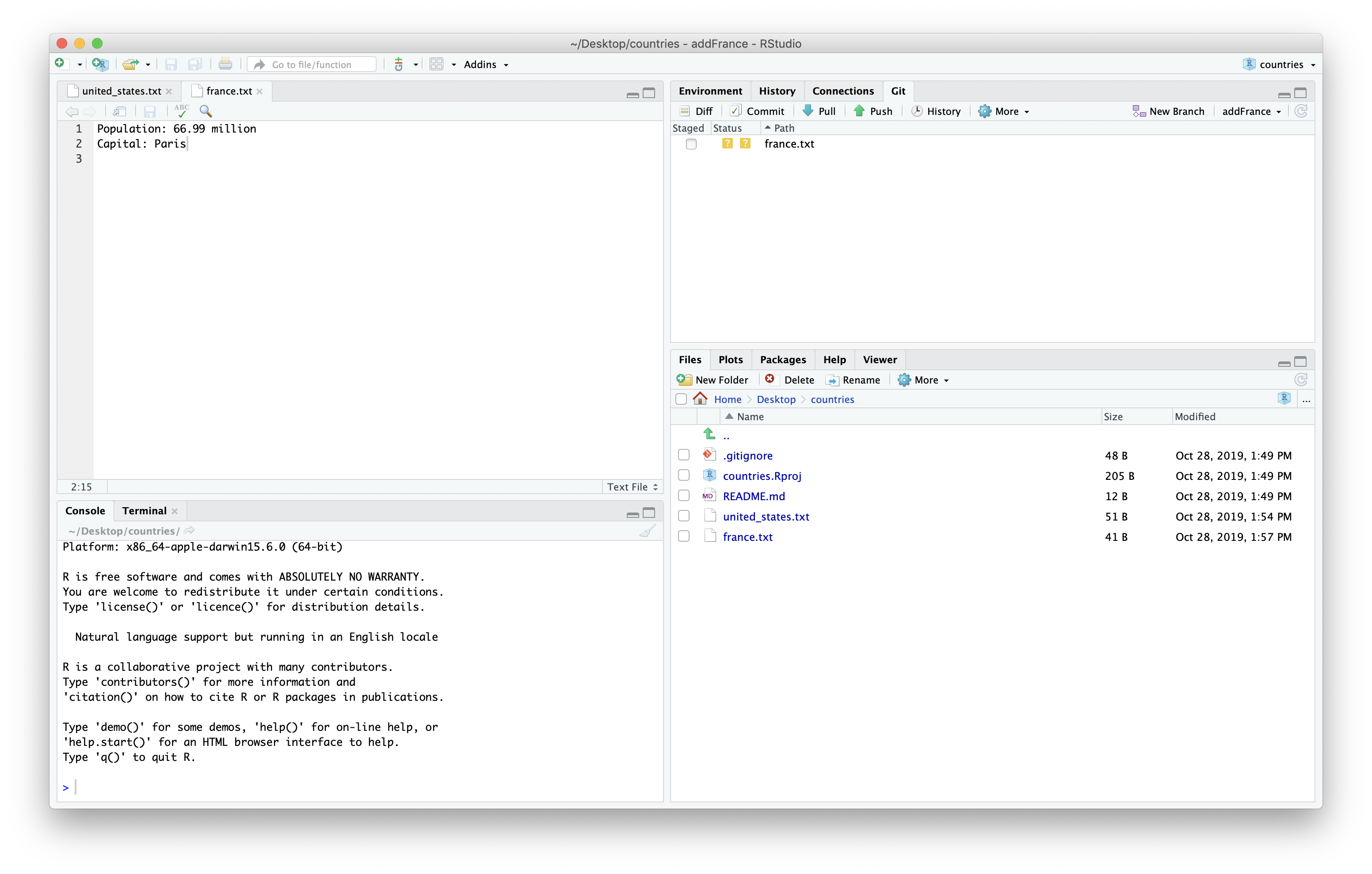
We can then save and stage the file.

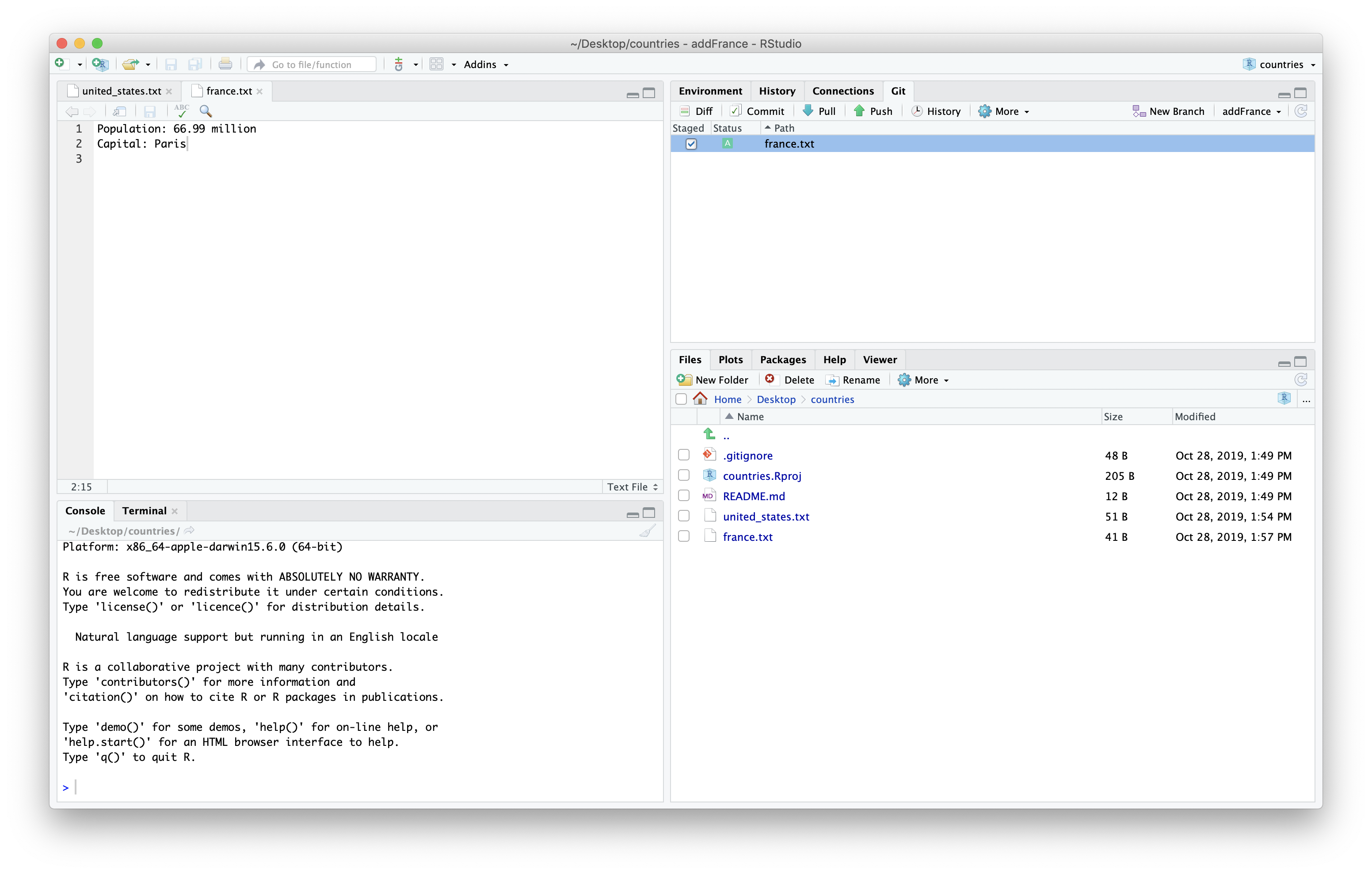
We can then commit the new file we added.

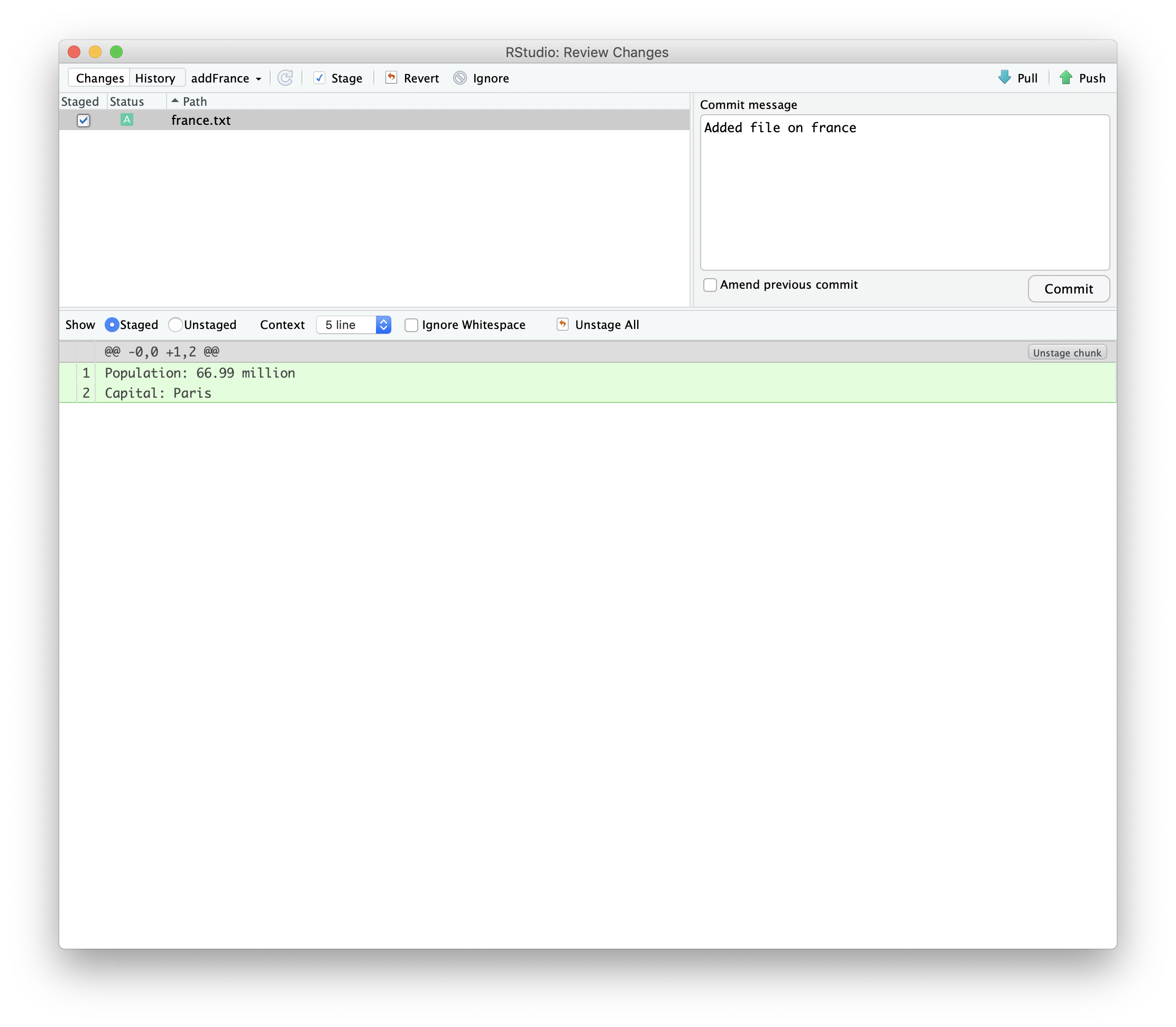
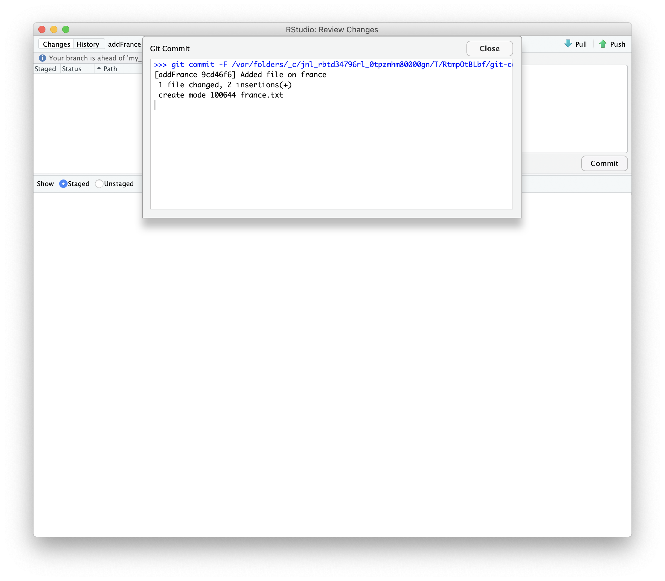
Then we can push those changes to our fork.

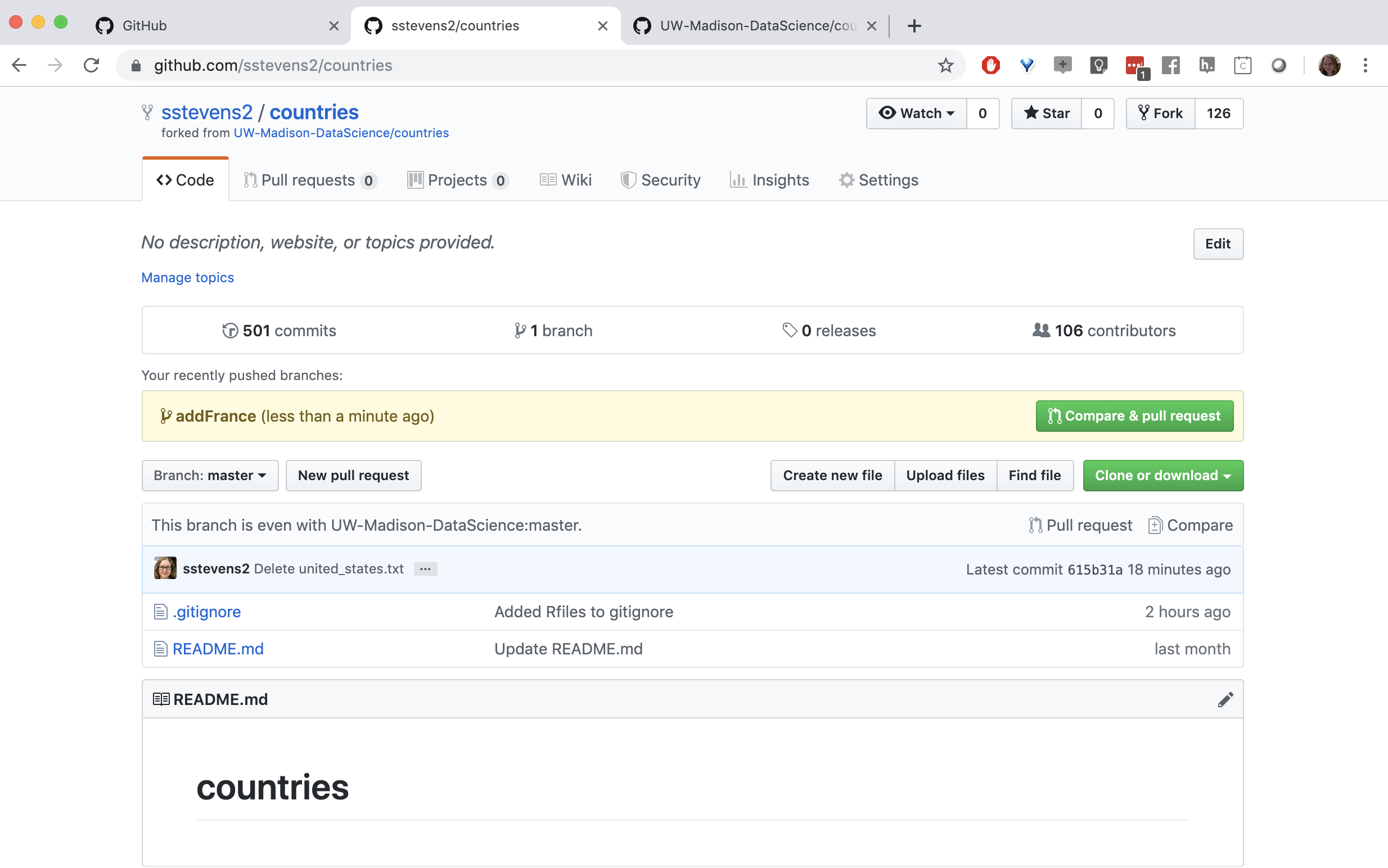
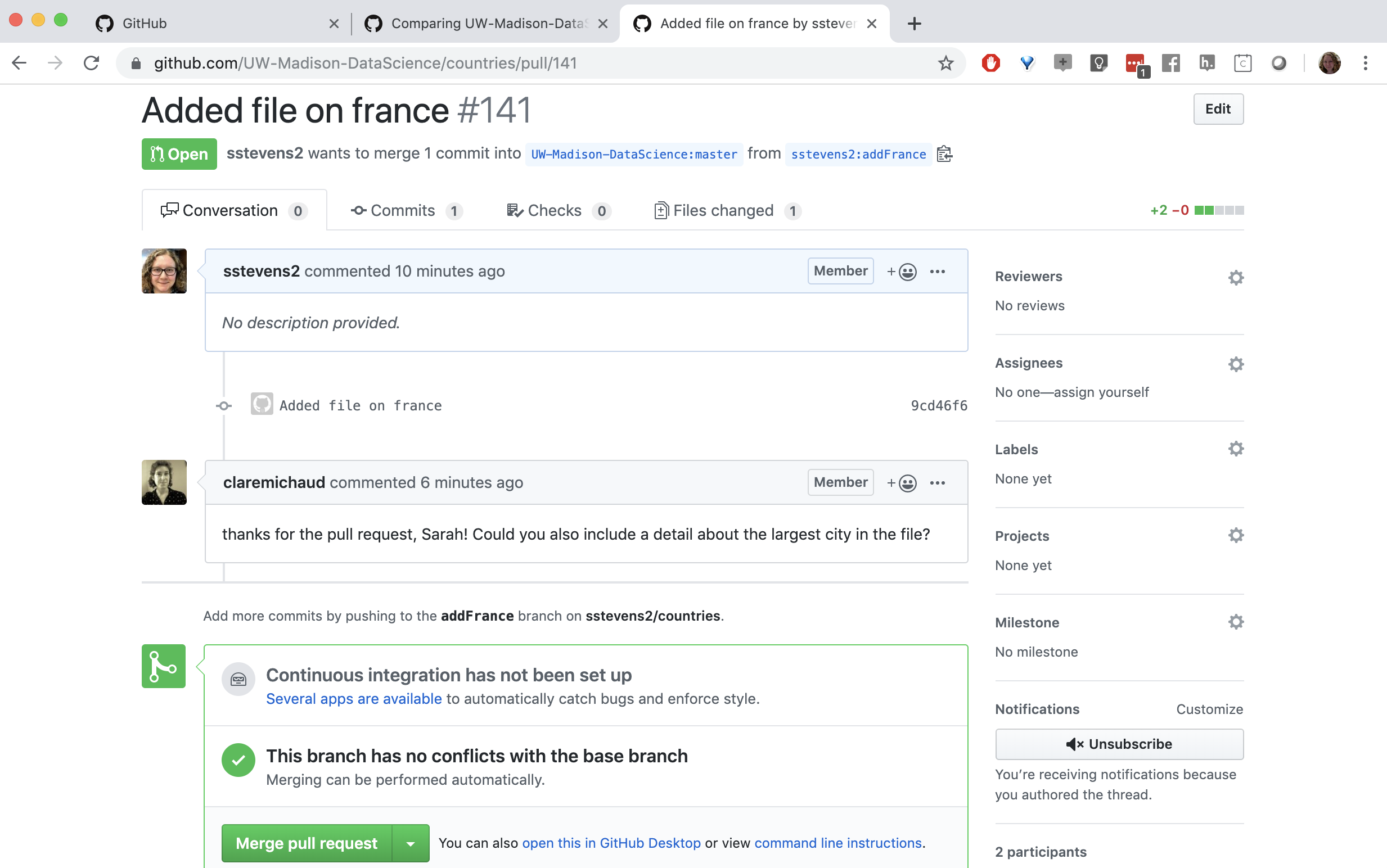
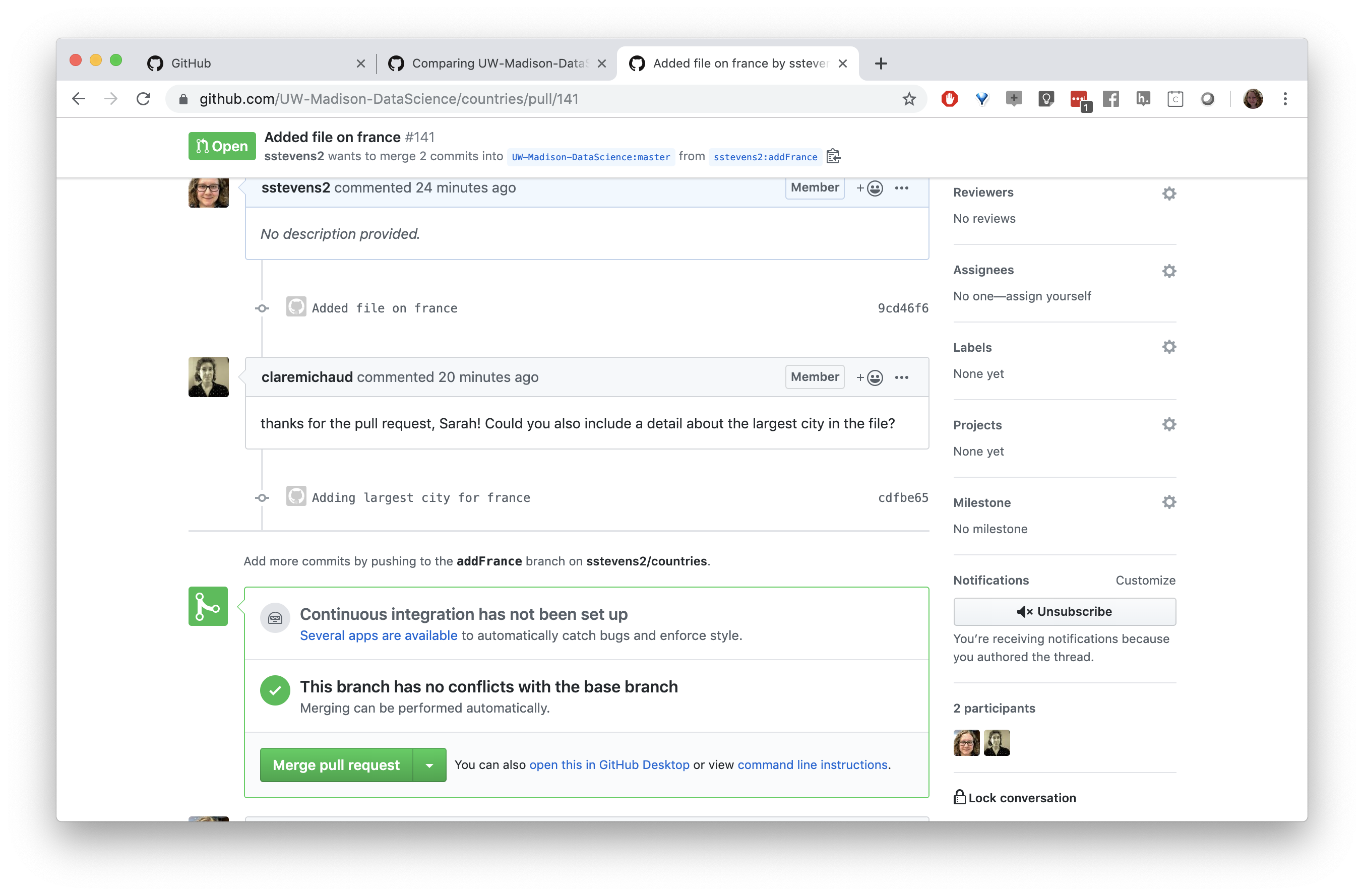
Now when we look at github we can see that there is a new branch. Github prompts us to compare and make a pull request.

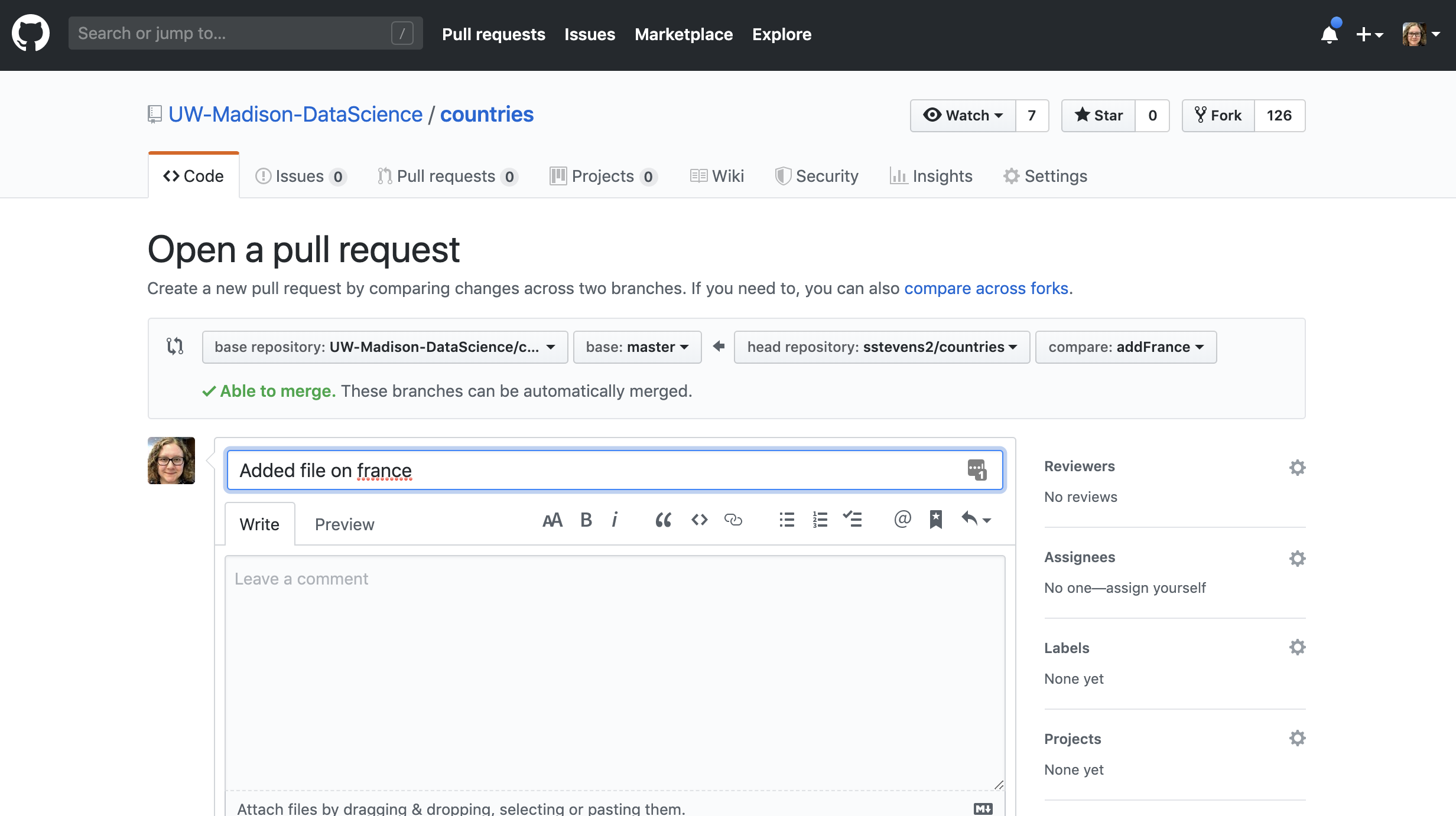
Then we can fill in the information to submit the pull request.

Then the person who owns the repo can look at the pull request and make edits.

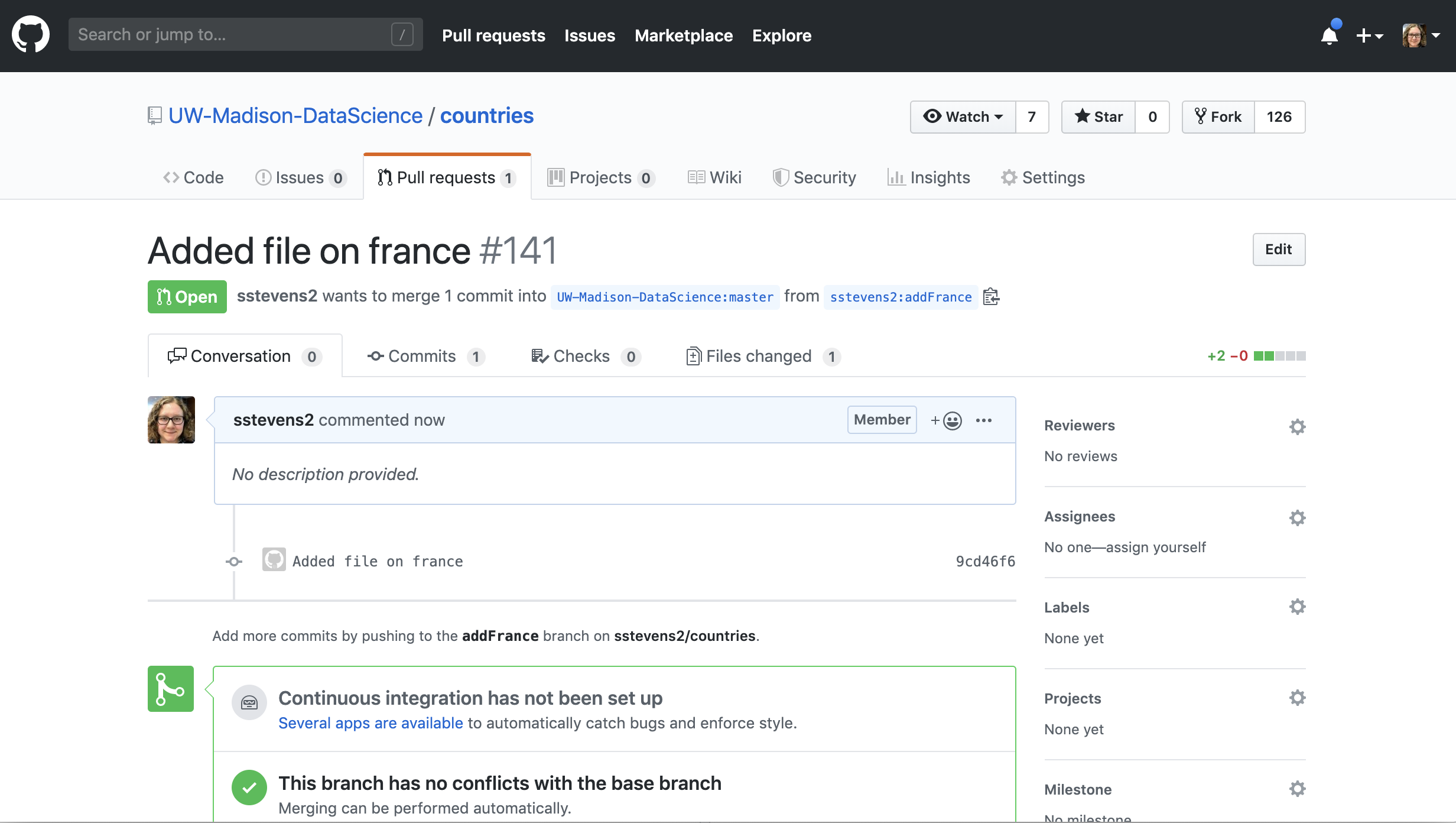
In our case our collaborator asked us if we could add the largest city to this file.

If we update the same branch we used in our pull request on our local machine and push it to our fork, it will update the pull request.

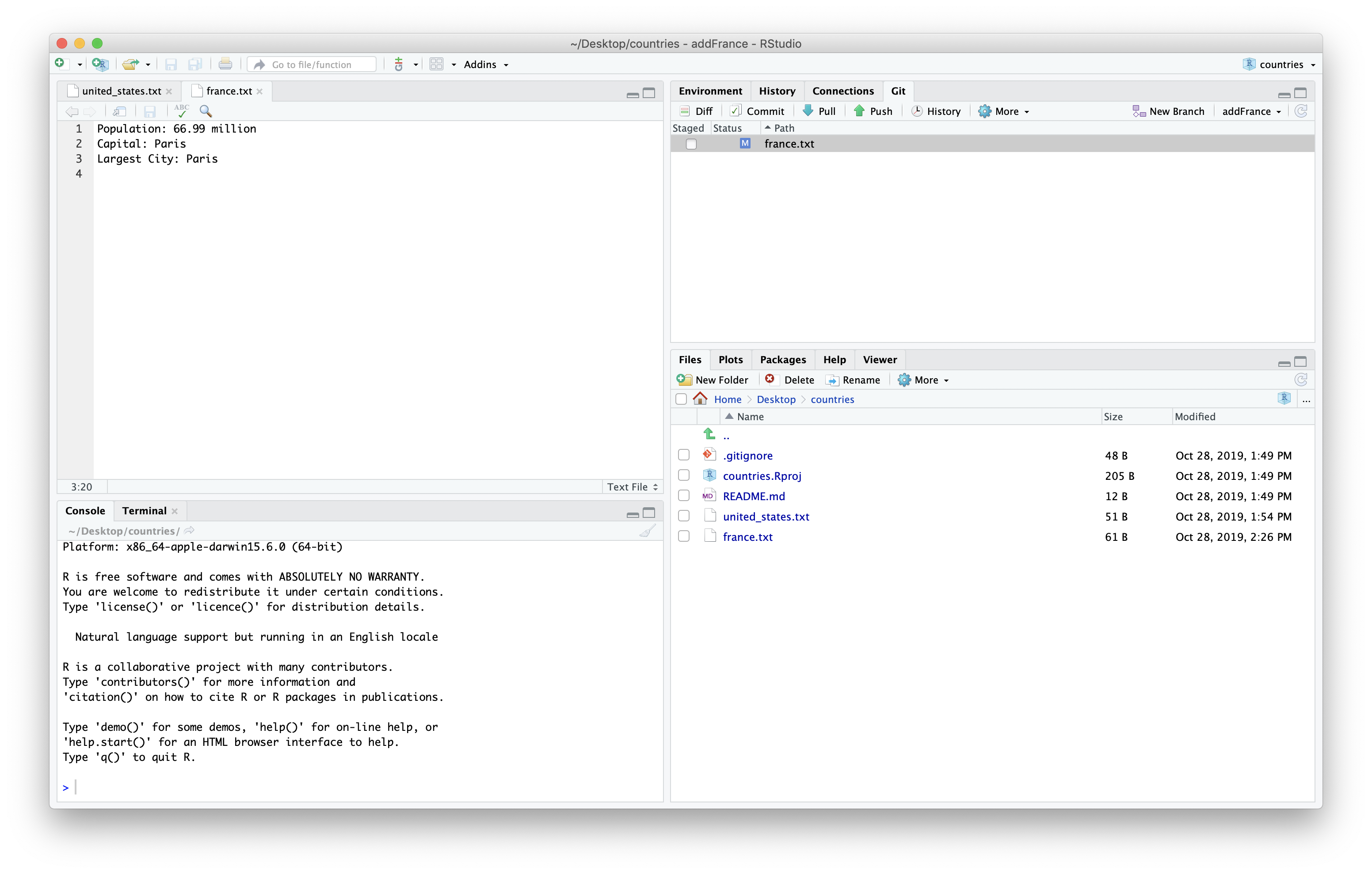
We then need to stage and commit the changes.

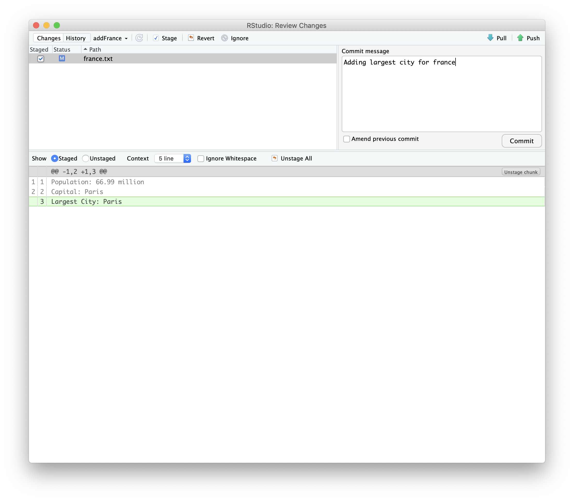
We can then push the changes to the repository.

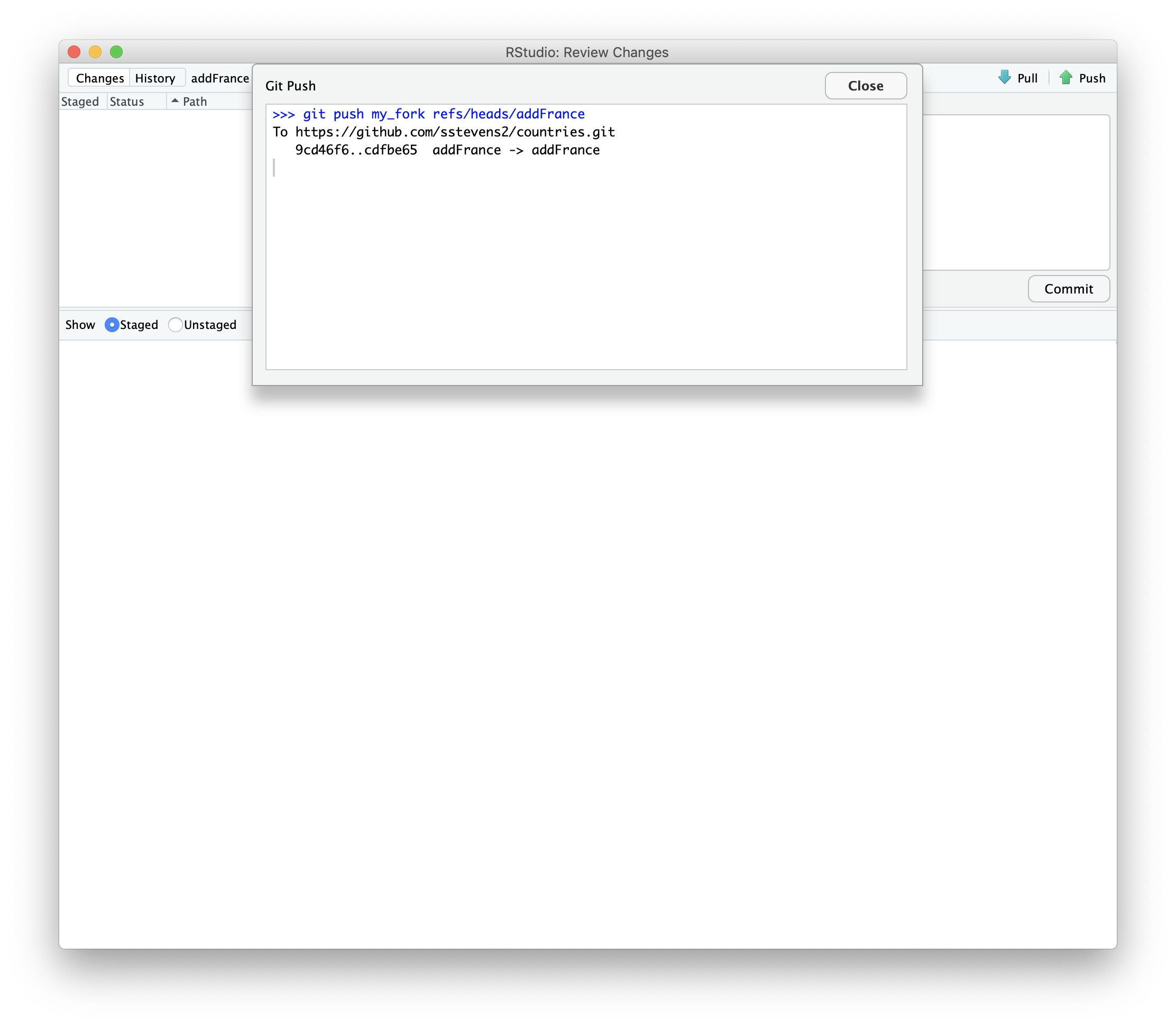
Now we can see the new commit on our pull request.

Key Points

• First key point. Brief Answer to questions. (FIXME)