Exploring high dimensional data
Overview
Teaching: 20 min
Exercises: 2 minQuestions
What is a high dimensional dataset?
Objectives
Define a dimension, index, and observation
Define, identify, and give examples of high dimensional datasets
Summarize the dimensionality of a given dataset
Introduction - what is high dimensional data?
What is data?
da·ta
/ˈdadə, ˈdādə/ noun “the quantities, characters, or symbols on which operations are performed by a computer”
—Oxford Languages
(how is data formatted? structured, semi-structured, unstructured: flat file, json, raw text)
There is a conversion to numerical representation happening here
A rectangular dataset: Original data set not rectangular, might require conversion that produces high dimensional rectangular data set.
We’re discussing structured, rectangular data only today.
What is a dimension?
di·men·sion
/dəˈmen(t)SH(ə)n, dīˈmen(t)SH(ə)n/
noun noun: dimension; plural noun: dimensions
- a measurable extent of some kind, such as length, breadth, depth, or height.
- an aspect or feature of a situation, problem, or thing.
—Oxford Languages
A Tabular/Rectangular Data Context

Each row is an observation, is a sample.

Each column is a feature, is a dimension.

The index is not a dimension.

A Dataset
- Some number of observations > 1
- every feature of an observation is a dimension
- the number of observations i.e. the index, is not a dimension
Examples of datasets with increasing dimensionality
1 D
- likert scale question (index: respondent_id, question value (-3 to 3)
2 D
- scatter plot (x, y)
- two question survey (index: respondent_id, q1 answer, q2 answer)
- data from temperature logger: (index: logged_value_id, time, value)
3 D
- surface (x, y, z)
- scatter plot with variable as size per point (x, y, size)
- 2d black and white image (x, y, pixel_value)
- moves log from a game of ‘battleship’ (index: move number, x-coord, y-coord, hit/miss)
- consecutive pulses of CP 1919 (time, x, y)

4 D
- surface plus coloration, (x, y, z, color_label)
- surface change over time (x, y, z, time)
30 D
- Brain connectivity analysis of 30 regions
20, 000 D
human gene expression e.g.

Exercise - Battleship moves:
discussion point is this 3d or 4d?
is the move number a dimension or an index?
move_id column (A-J) row (1-10) hit 0 A 1 False 1 J 10 True 2 C 7 False n … … Solution
3d: move_id is an index!
- order sequence matters but not the specific value of the move number
4d: move_id is a dimension!
- odd or even tells you which player is making which move
- order sequence is important, but when a specific moves get made might matter - what if you wanted to analyze moves as a function of game length?
There is always an index
- move_id is an index
- that doesn’t mean there is no information there
- you can perform some feature engineering with move_id
- this would up the dimensionality of the inital 3d dataset perhaps adding two more dimensions:
- player
- player’s move number
Exercise - Film:
consider a short, black and white, silent film, in 4K. It has the following properties:
- 1 minute long
- 25 frames per second
- 4K resolution i.e. 4096 × 2160.
- standard color depth 24 bits/pixel
Think of this film as a dataset, How many observations might there be?
Solution:
60 seconds x 25 frames per second = 1500 frames or ‘observations’. Is there another way to think about this?
Exercise: How many dimensions are there per observation?
Solution:
There are three dimensions per observation:
- pixel row (0-2159)
- pixel col (0-4095)
- pixel grey value (0-255)
Exercise: How many dimensions would there be if the film was longer, or shorter?
Solution:
- The number of dimensions would NOT change.
- There would simply be a greater or fewer number of ‘observations’
Exercise: How many dimensions would there be if the film was in color?
Solution:
4 dimensions.
There is an extra dimension per observation now.
- channel value (red, green, blue)
- pixel row (0-2159)
- pixel col (0-4095)
- pixel intensity (0-255)
Exercise: Titanic dataset
Look at the kaggle Titantic Dataset.
passenger_id pclass name sex age sibsp parch ticket fare cabin embarked boat body home.dest survived 1216 3 Smyth, Miss. Julia female 0 0 335432 7.7333 Q 13 1 699 3 Cacic, Mr. Luka male 38.0 0 0 315089 8.6625 S Croatia 0 1267 3 Van Impe, Mrs. Jean Baptiste (Rosalie Paula Govaert) female 30.0 1 1 345773 24.15 S 0 449 2 Hocking, Mrs. Elizabeth (Eliza Needs) female 54.0 1 3 29105 23.0 S 4 Cornwall / Akron, OH 1 576 2 Veal, Mr. James male 40.0 0 0 28221 13.0 S Barre, Co Washington, VT 0 What column is the index?
Solution:
PassengerId
Exercise: What columns are the dimensions?
Solution:
- pclass
- name
- sex
- age
- sibsp
- parch
- ticket
- fare
- cabin
- embarked
- survived
Exercise: how many dimensions are there?
Solution:
11
Exercise: Imagine building a model to predict survival on the titantic
- would you use every dimension?
- what makes a dimension useful?
- could you remove some dimensions?
- could you combine some dimensions?
- how would you combine those dimensions?
- do you have fewer dimensions after combining?
- do you have less information after combining?
Solution:
- No, some variables are poor predictors and can be ignored
- If it is (anti-)correlated with survival (in some context) i.e. has information.
- Yes any mostly null columns are not useful (add no information), any highly correlated columns also (no additional information)
- Yes
- Maybe add SibSp and Parch into one ‘family count’.
- Yes.
- Yes, but more data than if columns had been excluded.
High-Dimensional Data
What is high-dimensional data? Unfortunately, there isn’t a precise definition. Oftentimes, when people use the term, they are referring to data that has so many features that it is difficult to determine which features are relevant to the research question (dozens or more). In a modeling context, however, high-dimensional data is usually defined as a dataset where the number of features approaches or exceeds the number of observations.
The “curse of dimensionality” generally refers to the issues that arise when dealing with data in high-dimensional spaces, where distances between data points become less meaningful and the data becomes more sparse. This can lead to challenges in terms of computational complexity, overfitting in machine learning models, difficulties in visualization, and the need for specialized techniques to handle such data effectively.
So, whether the term “high-dimensional data” is used to describe datasets with a large number of features or datasets with a very high number of features, the underlying challenges related to dimensionality are usually concerned with the same issues of increased complexity and difficulties in analysis and modeling.
End of part 1
in part two we’ll start exploring a new dataset
Key Points
data can be anything - as long as you can represent it in a computer
A dimension is a feature in a dataset - i.e. a column, but NOT an index.
an index is not a dimension
The Ames housing dataset
Overview
Teaching: 45 min
Exercises: 2 minQuestions
Here we introduce the data we’ll be analyzing
Objectives
Intro to Ames Housing Dataset
Throughout this workshop, we will explore how to efficiently detect patterns and extract insights from high-dimensional data. We will focus on a widely accessible dataset known as the Ames housing data. This dataset will serve as a foundational example, allowing us to grasp the challenges and opportunities presented by high-dimensional data analysis.
Load the dataset
Here we load the dataset from the sklearn library, and see a preview
from sklearn.datasets import fetch_openml

# load the dataset
housing = fetch_openml(name="house_prices", as_frame=True, parser='auto')

df = housing.data.copy(deep=True) # create new DataFrame copy of original dataset
df = df.astype({'Id': int})       # set data type of Id to int
df = df.set_index('Id')           # set Id column to be the index of the DataFrame
df                                # evaluate result
| MSSubClass | MSZoning | LotFrontage | LotArea | Street | Alley | LotShape | LandContour | Utilities | LotConfig | ... | ScreenPorch | PoolArea | PoolQC | Fence | MiscFeature | MiscVal | MoSold | YrSold | SaleType | SaleCondition | |
|---|---|---|---|---|---|---|---|---|---|---|---|---|---|---|---|---|---|---|---|---|---|
| Id | |||||||||||||||||||||
| 1 | 60 | RL | 65.0 | 8450 | Pave | NaN | Reg | Lvl | AllPub | Inside | ... | 0 | 0 | NaN | NaN | NaN | 0 | 2 | 2008 | WD | Normal |
| 2 | 20 | RL | 80.0 | 9600 | Pave | NaN | Reg | Lvl | AllPub | FR2 | ... | 0 | 0 | NaN | NaN | NaN | 0 | 5 | 2007 | WD | Normal |
| 3 | 60 | RL | 68.0 | 11250 | Pave | NaN | IR1 | Lvl | AllPub | Inside | ... | 0 | 0 | NaN | NaN | NaN | 0 | 9 | 2008 | WD | Normal |
| 4 | 70 | RL | 60.0 | 9550 | Pave | NaN | IR1 | Lvl | AllPub | Corner | ... | 0 | 0 | NaN | NaN | NaN | 0 | 2 | 2006 | WD | Abnorml |
| 5 | 60 | RL | 84.0 | 14260 | Pave | NaN | IR1 | Lvl | AllPub | FR2 | ... | 0 | 0 | NaN | NaN | NaN | 0 | 12 | 2008 | WD | Normal |
| ... | ... | ... | ... | ... | ... | ... | ... | ... | ... | ... | ... | ... | ... | ... | ... | ... | ... | ... | ... | ... | ... |
| 1456 | 60 | RL | 62.0 | 7917 | Pave | NaN | Reg | Lvl | AllPub | Inside | ... | 0 | 0 | NaN | NaN | NaN | 0 | 8 | 2007 | WD | Normal |
| 1457 | 20 | RL | 85.0 | 13175 | Pave | NaN | Reg | Lvl | AllPub | Inside | ... | 0 | 0 | NaN | MnPrv | NaN | 0 | 2 | 2010 | WD | Normal |
| 1458 | 70 | RL | 66.0 | 9042 | Pave | NaN | Reg | Lvl | AllPub | Inside | ... | 0 | 0 | NaN | GdPrv | Shed | 2500 | 5 | 2010 | WD | Normal |
| 1459 | 20 | RL | 68.0 | 9717 | Pave | NaN | Reg | Lvl | AllPub | Inside | ... | 0 | 0 | NaN | NaN | NaN | 0 | 4 | 2010 | WD | Normal |
| 1460 | 20 | RL | 75.0 | 9937 | Pave | NaN | Reg | Lvl | AllPub | Inside | ... | 0 | 0 | NaN | NaN | NaN | 0 | 6 | 2008 | WD | Normal |
1460 rows × 79 columns
print(df.columns.tolist())
['MSSubClass', 'MSZoning', 'LotFrontage', 'LotArea', 'Street', 'Alley', 'LotShape', 'LandContour', 'Utilities', 'LotConfig', 'LandSlope', 'Neighborhood', 'Condition1', 'Condition2', 'BldgType', 'HouseStyle', 'OverallQual', 'OverallCond', 'YearBuilt', 'YearRemodAdd', 'RoofStyle', 'RoofMatl', 'Exterior1st', 'Exterior2nd', 'MasVnrType', 'MasVnrArea', 'ExterQual', 'ExterCond', 'Foundation', 'BsmtQual', 'BsmtCond', 'BsmtExposure', 'BsmtFinType1', 'BsmtFinSF1', 'BsmtFinType2', 'BsmtFinSF2', 'BsmtUnfSF', 'TotalBsmtSF', 'Heating', 'HeatingQC', 'CentralAir', 'Electrical', '1stFlrSF', '2ndFlrSF', 'LowQualFinSF', 'GrLivArea', 'BsmtFullBath', 'BsmtHalfBath', 'FullBath', 'HalfBath', 'BedroomAbvGr', 'KitchenAbvGr', 'KitchenQual', 'TotRmsAbvGrd', 'Functional', 'Fireplaces', 'FireplaceQu', 'GarageType', 'GarageYrBlt', 'GarageFinish', 'GarageCars', 'GarageArea', 'GarageQual', 'GarageCond', 'PavedDrive', 'WoodDeckSF', 'OpenPorchSF', 'EnclosedPorch', '3SsnPorch', 'ScreenPorch', 'PoolArea', 'PoolQC', 'Fence', 'MiscFeature', 'MiscVal', 'MoSold', 'YrSold', 'SaleType', 'SaleCondition']
Dataset Preview Exercises
How many features are there?
Solution
79
EXERCISE: How many observations are there?
Solution
1460
EXERCISE: What are all the feature names?
Solution
print(df.columns.tolist())['MSSubClass', 'MSZoning', 'LotFrontage', 'LotArea', 'Street', 'Alley', 'LotShape', 'LandContour', 'Utilities', 'LotConfig', 'LandSlope', 'Neighborhood', 'Condition1', 'Condition2', 'BldgType', 'HouseStyle', 'OverallQual', 'OverallCond', 'YearBuilt', 'YearRemodAdd', 'RoofStyle', 'RoofMatl', 'Exterior1st', 'Exterior2nd', 'MasVnrType', 'MasVnrArea', 'ExterQual', 'ExterCond', 'Foundation', 'BsmtQual', 'BsmtCond', 'BsmtExposure', 'BsmtFinType1', 'BsmtFinSF1', 'BsmtFinType2', 'BsmtFinSF2', 'BsmtUnfSF', 'TotalBsmtSF', 'Heating', 'HeatingQC', 'CentralAir', 'Electrical', '1stFlrSF', '2ndFlrSF', 'LowQualFinSF', 'GrLivArea', 'BsmtFullBath', 'BsmtHalfBath', 'FullBath', 'HalfBath', 'BedroomAbvGr', 'KitchenAbvGr', 'KitchenQual', 'TotRmsAbvGrd', 'Functional', 'Fireplaces', 'FireplaceQu', 'GarageType', 'GarageYrBlt', 'GarageFinish', 'GarageCars', 'GarageArea', 'GarageQual', 'GarageCond', 'PavedDrive', 'WoodDeckSF', 'OpenPorchSF', 'EnclosedPorch', '3SsnPorch', 'ScreenPorch', 'PoolArea', 'PoolQC', 'Fence', 'MiscFeature', 'MiscVal', 'MoSold', 'YrSold', 'SaleType', 'SaleCondition']EXERCISE_END
How do I find out what these features mean?
Read the Data Dictionary
from IPython.display import display, Pretty

# the housing object we created in step one above contains a Data Dictionary for the Dataset
display(Pretty(housing.DESCR))
Ask a home buyer to describe their dream house, and they probably won’t begin with the height of the basement ceiling or the proximity to an east-west railroad. But this playground competition’s dataset proves that much more influences price negotiations than the number of bedrooms or a white-picket fence.
With 79 explanatory variables describing (almost) every aspect of residential homes in Ames, Iowa, this competition challenges you to predict the final price of each home.
MSSubClass: Identifies the type of dwelling involved in the sale.
20 1-STORY 1946 & NEWER ALL STYLES 30 1-STORY 1945 & OLDER 40 1-STORY W/FINISHED ATTIC ALL AGES 45 1-1/2 STORY - UNFINISHED ALL AGES 50 1-1/2 STORY FINISHED ALL AGES 60 2-STORY 1946 & NEWER 70 2-STORY 1945 & OLDER 75 2-1/2 STORY ALL AGES 80 SPLIT OR MULTI-LEVEL 85 SPLIT FOYER 90 DUPLEX - ALL STYLES AND AGES 120 1-STORY PUD (Planned Unit Development) - 1946 & NEWER 150 1-1/2 STORY PUD - ALL AGES 160 2-STORY PUD - 1946 & NEWER 180 PUD - MULTILEVEL - INCL SPLIT LEV/FOYER 190 2 FAMILY CONVERSION - ALL STYLES AND AGES
MSZoning: Identifies the general zoning classification of the sale.
A Agriculture C Commercial FV Floating Village Residential I Industrial RH Residential High Density RL Residential Low Density RP Residential Low Density Park RM Residential Medium Density
LotFrontage: Linear feet of street connected to property
LotArea: Lot size in square feet
Street: Type of road access to property
Grvl Gravel Pave Paved
Alley: Type of alley access to property
Grvl Gravel Pave Paved NA No alley access
LotShape: General shape of property
Reg Regular IR1 Slightly irregular IR2 Moderately Irregular IR3 Irregular
LandContour: Flatness of the property
Lvl Near Flat/Level Bnk Banked - Quick and significant rise from street grade to building HLS Hillside - Significant slope from side to side Low Depression
Utilities: Type of utilities available
AllPub All public Utilities (E,G,W,& S) NoSewr Electricity, Gas, and Water (Septic Tank) NoSeWa Electricity and Gas Only ELO Electricity only
LotConfig: Lot configuration
Inside Inside lot Corner Corner lot CulDSac Cul-de-sac FR2 Frontage on 2 sides of property FR3 Frontage on 3 sides of property
LandSlope: Slope of property
Gtl Gentle slope Mod Moderate Slope Sev Severe Slope
Neighborhood: Physical locations within Ames city limits
Blmngtn Bloomington Heights Blueste Bluestem BrDale Briardale BrkSide Brookside ClearCr Clear Creek CollgCr College Creek Crawfor Crawford Edwards Edwards Gilbert Gilbert IDOTRR Iowa DOT and Rail Road MeadowV Meadow Village Mitchel Mitchell Names North Ames NoRidge Northridge NPkVill Northpark Villa NridgHt Northridge Heights NWAmes Northwest Ames OldTown Old Town SWISU South & West of Iowa State University Sawyer Sawyer SawyerW Sawyer West Somerst Somerset StoneBr Stone Brook Timber Timberland Veenker Veenker
Condition1: Proximity to various conditions
Artery Adjacent to arterial street Feedr Adjacent to feeder street Norm Normal RRNn Within 200’ of North-South Railroad RRAn Adjacent to North-South Railroad PosN Near positive off-site feature–park, greenbelt, etc. PosA Adjacent to postive off-site feature RRNe Within 200’ of East-West Railroad RRAe Adjacent to East-West Railroad
Condition2: Proximity to various conditions (if more than one is present)
Artery Adjacent to arterial street Feedr Adjacent to feeder street Norm Normal RRNn Within 200’ of North-South Railroad RRAn Adjacent to North-South Railroad PosN Near positive off-site feature–park, greenbelt, etc. PosA Adjacent to postive off-site feature RRNe Within 200’ of East-West Railroad RRAe Adjacent to East-West Railroad
BldgType: Type of dwelling
1Fam Single-family Detached 2FmCon Two-family Conversion; originally built as one-family dwelling Duplx Duplex TwnhsE Townhouse End Unit TwnhsI Townhouse Inside Unit
HouseStyle: Style of dwelling
1Story One story 1.5Fin One and one-half story: 2nd level finished 1.5Unf One and one-half story: 2nd level unfinished 2Story Two story 2.5Fin Two and one-half story: 2nd level finished 2.5Unf Two and one-half story: 2nd level unfinished SFoyer Split Foyer SLvl Split Level
OverallQual: Rates the overall material and finish of the house
10 Very Excellent 9 Excellent 8 Very Good 7 Good 6 Above Average 5 Average 4 Below Average 3 Fair 2 Poor 1 Very Poor
OverallCond: Rates the overall condition of the house
10 Very Excellent 9 Excellent 8 Very Good 7 Good 6 Above Average 5 Average 4 Below Average 3 Fair 2 Poor 1 Very Poor
YearBuilt: Original construction date
YearRemodAdd: Remodel date (same as construction date if no remodeling or additions)
RoofStyle: Type of roof
Flat Flat Gable Gable Gambrel Gabrel (Barn) Hip Hip Mansard Mansard Shed Shed
RoofMatl: Roof material
ClyTile Clay or Tile CompShg Standard (Composite) Shingle Membran Membrane Metal Metal Roll Roll Tar&Grv Gravel & Tar WdShake Wood Shakes WdShngl Wood Shingles
Exterior1st: Exterior covering on house
AsbShng Asbestos Shingles AsphShn Asphalt Shingles BrkComm Brick Common BrkFace Brick Face CBlock Cinder Block CemntBd Cement Board HdBoard Hard Board ImStucc Imitation Stucco MetalSd Metal Siding Other Other Plywood Plywood PreCast PreCast Stone Stone Stucco Stucco VinylSd Vinyl Siding Wd Sdng Wood Siding WdShing Wood Shingles
Exterior2nd: Exterior covering on house (if more than one material)
AsbShng Asbestos Shingles AsphShn Asphalt Shingles BrkComm Brick Common BrkFace Brick Face CBlock Cinder Block CemntBd Cement Board HdBoard Hard Board ImStucc Imitation Stucco MetalSd Metal Siding Other Other Plywood Plywood PreCast PreCast Stone Stone Stucco Stucco VinylSd Vinyl Siding Wd Sdng Wood Siding WdShing Wood Shingles
MasVnrType: Masonry veneer type
BrkCmn Brick Common BrkFace Brick Face CBlock Cinder Block None None Stone Stone
MasVnrArea: Masonry veneer area in square feet
ExterQual: Evaluates the quality of the material on the exterior
Ex Excellent Gd Good TA Average/Typical Fa Fair Po Poor
ExterCond: Evaluates the present condition of the material on the exterior
Ex Excellent Gd Good TA Average/Typical Fa Fair Po Poor
Foundation: Type of foundation
BrkTil Brick & Tile CBlock Cinder Block PConc Poured Contrete Slab Slab Stone Stone Wood Wood
BsmtQual: Evaluates the height of the basement
Ex Excellent (100+ inches) Gd Good (90-99 inches) TA Typical (80-89 inches) Fa Fair (70-79 inches) Po Poor (<70 inches NA No Basement
BsmtCond: Evaluates the general condition of the basement
Ex Excellent Gd Good TA Typical - slight dampness allowed Fa Fair - dampness or some cracking or settling Po Poor - Severe cracking, settling, or wetness NA No Basement
BsmtExposure: Refers to walkout or garden level walls
Gd Good Exposure Av Average Exposure (split levels or foyers typically score average or above) Mn Mimimum Exposure No No Exposure NA No Basement
BsmtFinType1: Rating of basement finished area
GLQ Good Living Quarters ALQ Average Living Quarters BLQ Below Average Living Quarters Rec Average Rec Room LwQ Low Quality Unf Unfinshed NA No Basement
BsmtFinSF1: Type 1 finished square feet
BsmtFinType2: Rating of basement finished area (if multiple types)
GLQ Good Living Quarters ALQ Average Living Quarters BLQ Below Average Living Quarters Rec Average Rec Room LwQ Low Quality Unf Unfinshed NA No Basement
BsmtFinSF2: Type 2 finished square feet
BsmtUnfSF: Unfinished square feet of basement area
TotalBsmtSF: Total square feet of basement area
Heating: Type of heating
Floor Floor Furnace GasA Gas forced warm air furnace GasW Gas hot water or steam heat Grav Gravity furnace OthW Hot water or steam heat other than gas Wall Wall furnace
HeatingQC: Heating quality and condition
Ex Excellent Gd Good TA Average/Typical Fa Fair Po Poor
CentralAir: Central air conditioning
N No Y Yes
Electrical: Electrical system
SBrkr Standard Circuit Breakers & Romex FuseA Fuse Box over 60 AMP and all Romex wiring (Average) FuseF 60 AMP Fuse Box and mostly Romex wiring (Fair) FuseP 60 AMP Fuse Box and mostly knob & tube wiring (poor) Mix Mixed
1stFlrSF: First Floor square feet
2ndFlrSF: Second floor square feet
LowQualFinSF: Low quality finished square feet (all floors)
GrLivArea: Above grade (ground) living area square feet
BsmtFullBath: Basement full bathrooms
BsmtHalfBath: Basement half bathrooms
FullBath: Full bathrooms above grade
HalfBath: Half baths above grade
Bedroom: Bedrooms above grade (does NOT include basement bedrooms)
Kitchen: Kitchens above grade
KitchenQual: Kitchen quality
Ex Excellent Gd Good TA Typical/Average Fa Fair Po Poor
TotRmsAbvGrd: Total rooms above grade (does not include bathrooms)
Functional: Home functionality (Assume typical unless deductions are warranted)
Typ Typical Functionality Min1 Minor Deductions 1 Min2 Minor Deductions 2 Mod Moderate Deductions Maj1 Major Deductions 1 Maj2 Major Deductions 2 Sev Severely Damaged Sal Salvage only
Fireplaces: Number of fireplaces
FireplaceQu: Fireplace quality
Ex Excellent - Exceptional Masonry Fireplace Gd Good - Masonry Fireplace in main level TA Average - Prefabricated Fireplace in main living area or Masonry Fireplace in basement Fa Fair - Prefabricated Fireplace in basement Po Poor - Ben Franklin Stove NA No Fireplace
GarageType: Garage location
2Types More than one type of garage Attchd Attached to home Basment Basement Garage BuiltIn Built-In (Garage part of house - typically has room above garage) CarPort Car Port Detchd Detached from home NA No Garage
GarageYrBlt: Year garage was built
GarageFinish: Interior finish of the garage
Fin Finished RFn Rough Finished Unf Unfinished NA No Garage
GarageCars: Size of garage in car capacity
GarageArea: Size of garage in square feet
GarageQual: Garage quality
Ex Excellent Gd Good TA Typical/Average Fa Fair Po Poor NA No Garage
GarageCond: Garage condition
Ex Excellent Gd Good TA Typical/Average Fa Fair Po Poor NA No Garage
PavedDrive: Paved driveway
Y Paved P Partial Pavement N Dirt/Gravel
WoodDeckSF: Wood deck area in square feet
OpenPorchSF: Open porch area in square feet
EnclosedPorch: Enclosed porch area in square feet
3SsnPorch: Three season porch area in square feet
ScreenPorch: Screen porch area in square feet
PoolArea: Pool area in square feet
PoolQC: Pool quality
Ex Excellent Gd Good TA Average/Typical Fa Fair NA No Pool
Fence: Fence quality
GdPrv Good Privacy MnPrv Minimum Privacy GdWo Good Wood MnWw Minimum Wood/Wire NA No Fence
MiscFeature: Miscellaneous feature not covered in other categories
Elev Elevator Gar2 2nd Garage (if not described in garage section) Othr Other Shed Shed (over 100 SF) TenC Tennis Court NA None
MiscVal: $Value of miscellaneous feature
MoSold: Month Sold (MM)
YrSold: Year Sold (YYYY)
SaleType: Type of sale
WD Warranty Deed - Conventional CWD Warranty Deed - Cash VWD Warranty Deed - VA Loan New Home just constructed and sold COD Court Officer Deed/Estate Con Contract 15% Down payment regular terms ConLw Contract Low Down payment and low interest ConLI Contract Low Interest ConLD Contract Low Down Oth Other
SaleCondition: Condition of sale
Normal Normal Sale Abnorml Abnormal Sale - trade, foreclosure, short sale AdjLand Adjoining Land Purchase Alloca Allocation - two linked properties with separate deeds, typically condo with a garage unit Family Sale between family members Partial Home was not completed when last assessed (associated with New Homes)
Downloaded from openml.org.
Feature Exercises
EXERCISE_START
What information is represented by BsmtFinType2?
Solution
Rating of basement finished area (if multiple types)
EXERCISE_START
What type of variable is BsmtFinType2 (categorical or numeric, then nominal/ordinal or discrete/continuous)?
Solution
categorical, ordinate
EXERCISE_START
What information is represented by GrLivArea?
Solution
Above grade (ground) living area square feet
EXERCISE_START
What type of variable is GrLivArea? (categorical or numeric, then nominal/ordinal or discrete/continuous)?
Solution
numeric, discrete
Load the Target (Response) Variable - Housing Price
import pandas as pd

housing_price_df = pd.DataFrame(housing.target) # load data into dataframe
housing_price_df.describe()                     # create numeric summary of that data
| SalePrice | |
|---|---|
| count | 1460.000000 |
| mean | 180921.195890 |
| std | 79442.502883 |
| min | 34900.000000 |
| 25% | 129975.000000 |
| 50% | 163000.000000 |
| 75% | 214000.000000 |
| max | 755000.000000 |
Price Exercises
EXERCISE_START
What is the range of housing prices in the dataset?
Solution
min: $34,900, max: $755,000
EXERCISE_START
Are the price data skewed? What distribution might you expect?
Solution
yes, positive/right handed skew. Expect positive/right handed skew from a long tail to outlier high values
Plot housing price values
import helper_functions
helper_functions.plot_salesprice(
    housing_price_df,
    # ylog=True
)
Summary
In this session we:
- Introduced the Ames Housing Dataset
- Determined the number of features and observations
- Understood some variables
- Viewed the ‘target variable’: SalePrice
Key Points
Predictive vs. explanatory regression
Overview
Teaching: 45 min
Exercises: 2 minQuestions
What are the two different goals to keep in mind when fitting machine learning models?
What kinds of questions can be answered using linear regresion?
How can we evaluate a model’s ability to capture a true signal/relationship in the data versus spurious noise?
Objectives
Review structure and goals of linear regression
Know when to use different model evaluation metrics for different modeling goals
Learn how to train and evaluate a predictive machine learning model
Understand how to detect underfitting and overfitting in a machine learning model
Linear Regression
Linear regression is powerful technique that is often used to understand whether and how certain predictor variables (e.g., garage size, year built, etc.) in a dataset linearly relate to some target variable (e.g., house sale prices). Starting with linear models when working with high-dimensional data can offer several advantages including:
-
Simplicity and Interpretability: Linear models, such as linear regression, are relatively simple and interpretable. They provide a clear understanding of how each predictor variable contributes to the outcome, which can be especially valuable in exploratory analysis.
-
Baseline Understanding: Linear models can serve as a baseline for assessing the predictive power of individual features. This baseline helps you understand which features have a significant impact on the target variable and which ones might be less influential.
-
Feature Selection: Linear models can help you identify relevant features by looking at the estimated coefficients. Features with large coefficients are likely to have a stronger impact on the outcome, while those with small coefficients might have negligible effects
While linear models have their merits, it’s important to recognize that they might not capture complex (nonlinear) relationships present in the data. However, they are often the best option available when working in a high-dimensional context unless data is extremely limited.
Goals of Linear Regression
By fitting linear models to the Ames housing dataset, we can…
- Predict: Use predictive modeling to predict hypothetical/future sale prices based on observed values of the predictor variables in our dataset (e.g., garage size, year built, etc.).
- Explain: Use statistics to make scientific claims concerning which predictor variables have a significant impact on sale price — the target variable (a.k.a. response / dependent variable)
Terminology note: “target” and “predictor” synonyms
- Predictor = independent variable = feature = regressor
- Target = dependent variable = response = outcome
In this workshop, we will explore how we can exploit well-established machine learning methods, including feature selection, and regularization techniques (more on these terms later), to achieve both of the above goals on high-dimensional datasets.
To predict or explain. That is the question.
When trying to model data you use in your work, which goal is typically more prevalent? Do you typically care more about (1) accurately predicting some target variable or (2) making scientific claims concerning the existence of certain relationships between variables?
Solution
In a research setting, explaining relationships typically takes higher priority over predicting since explainations hold high value in science, but both goals are sometimes relevant. In industry, the reverse is typically true as many industry applications place predictive accuracy above explainability. We will explore how these goals align and sometimes diverge from one another throughout the remaining lessons.
Predicting housing prices with a single predictor
We’ll start with the first goal: prediction. How can we use regression models to predict housing sale prices? For clarity, we will begin this question through the lens of simple univariate regression models.
General procedure for fitting and evaluating predictive models
We’ll follow this general procedure to fit and evaluate predictive models:
- Extract predictor(s), X, and target, y, variables
- Preprocess the data: check for NaNs and extreme sparsity
- Visualize the relationship between X and y
- Transform target variable, if necessary, to get a linear relationship between predictors
- Train/test split the data
- Fit the model to the training data
-
Evaluate model
a. Plot the data vs predictions - qualitative assessment
b. Measure train/test set errors and check for signs of underfitting or overfitting
We’ll start by loading in the Ames housing data as we have done previously in this workshop.
from sklearn.datasets import fetch_openml
housing = fetch_openml(name="house_prices", as_frame=True, parser='auto') #
1) Extract predictor variable and target variable from dataframe
Next, we’ll extract the two variables we’ll use for our model — the target variable that we’ll attempt to predict (SalePrice), and a single predictor variable that will be used to predict the target variable. For this example, we’ll explore how well the “OverallQual” variable (i.e., the predictor variable) can predict sale prices.
OverallQual: Rates the overall material and finish of the house
   10	Very Excellent
   1	Very Poor
# Extract x (predictor) and y (target)
y = housing['target']
predictor = 'OverallQual'
x = housing['data'][predictor]
2) Preprocess the data
# remove columns with nans or containing > 97% constant values (typically 0's)
from preprocessing import remove_bad_cols
x_good = remove_bad_cols(x, 95)
0 columns removed, 1 remaining.
3) Visualize the relationship between x and y
Before fitting any models in a univariate context, we should first explore the data to get a sense for the relationship between the predictor variable, “OverallQual”, and the response variable, “SalePrice”. If this relationship does not look linear, we won’t be able to fit a good linear model (i.e., a model with low average prediction error in a predictive modeling context) to the data.
import matplotlib.pyplot as plt
plt.scatter(x,y, alpha=.1)
plt.xlabel(predictor)
plt.ylabel('Sale Price');
# plt.savefig('..//fig//regression//intro//scatterplot_x_vs_salePrice.png', bbox_inches='tight', dpi=300, facecolor='white');

4) Transform target variable, if necessary
Unfortunately, sale price appears to grow almost exponentially—not linearly—with the predictor variable. Any line we draw through this data cloud is going to fail in capturing the true trend we see here.
Log scaling
How can we remedy this situation? One common approach is to log transform the target variable. We’ll convert the “SalePrice” variable to its logarithmic form by using the math.log() function. Pandas has a special function called apply which can apply an operation to every item in a series by using the statement y.apply(math.log), where y is a pandas series.
import numpy as np
y_log = y.apply(np.log)
plt.scatter(x,y_log, alpha=.1)
plt.xlabel(predictor)
plt.ylabel('Sale Price');
# plt.savefig('..//fig//regression//intro//scatterplot_x_vs_logSalePrice.png', bbox_inches='tight', dpi=300, facecolor='white')

This plot looks much better than the previous one. That is, the trend between OverallQual and log(SalePrice) appears fairly linear. Whether or not it is sufficiently linear can be addressed when we evaluate the model’s performance later.
5) Train/test split
Next, we will prepare two subsets of our data to be used for model-fitting and model evaluation. This process is standard for any predictive modeling task that involves a model “learning” from observed data (e.g., fitting a line to the observed data).
During the model-fitting step, we use a subset of the data referred to as training data to estimate the model’s coefficients (the slope of the model). The univariate model will find a line of best fit through this data.
Next, we can assess the model’s ability to generalize to new datasets by measuring its performance on the remaining, unseen data. This subset of data is referred to as the test data or holdout set. By evaluating the model on the test set, which was not used during training, we can obtain an unbiased estimate of the model’s performance.
If we were to evaluate the model solely on the training data, it could lead to overfitting. Overfitting occurs when the model learns the noise and specific patterns of the training data too well, resulting in poor performance on new data. By using a separate test set, we can identify if the model has overfit the training data and assess its ability to generalize to unseen samples. While overfitting is typically not likely to occur when using only a single predictor variable, it is still a good idea to use a train/test split when fitting univariate models. This can help in detecting unanticipated issues with the data, such as missing values, outliers, or other anomalies that affect the model’s behavior.

The below code will split our dataset into a training dataset containing 2/3 of the samples, and a test set containing the remaining 1/3 of the data. We’ll discuss these different subsets in more detail in just a bit.
from sklearn.model_selection import train_test_split

x_train, x_test, y_train, y_test = train_test_split(x, y_log,
                                                    test_size=0.33,
                                                    random_state=0)

print(x_train.shape)
print(x_test.shape)
(978,)
(482,)
Reshape single-var predictor matrix in preparation for model-fitting step (requires a 2-D representation)
x_train = x_train.values.reshape(-1,1)
x_test = x_test.values.reshape(-1,1)
print(x_train.shape)
print(x_test.shape)
(978, 1)
(482, 1)
6) Fit the model to the training dataset
During the model fitting step, we use a subset of the data referred to as training data to estimate the model’s coefficients. The univariate model will find a line of best fit through this data.
The sklearn library
When fitting linear models solely for predictive purposes, the scikit-learn or “sklearn” library is typically used. Sklearn offers a broad spectrum of machine learning algorithms beyond linear regression. Having multiple algorithms available in the same library allows you to switch between different models easily and experiment with various techniques without switching libraries. Sklearn is also optimized for performance and efficiency, which is beneficial when working with large datasets. It can efficiently handle large-scale linear regression tasks, and if needed, you can leverage tools like NumPy and SciPy, which are well-integrated with scikit-learn for faster numerical computations.
from sklearn.linear_model import LinearRegression
reg = LinearRegression().fit(x_train,y_train)
7) Evaluate model
a) Plot the data vs predictions - qualitative assessment
y_pred_train=reg.predict(x_train)
y_pred_test=reg.predict(x_test)
from regression_predict_sklearn import plot_train_test_predictions

help(plot_train_test_predictions)
Help on function plot_train_test_predictions in module regression_predict_sklearn:

plot_train_test_predictions(predictors: List[str], X_train: Union[numpy.ndarray, pandas.core.series.Series, pandas.core.frame.DataFrame], X_test: Union[numpy.ndarray, pandas.core.series.Series, pandas.core.frame.DataFrame], y_train: Union[numpy.ndarray, pandas.core.series.Series], y_test: Union[numpy.ndarray, pandas.core.series.Series], y_pred_train: Union[numpy.ndarray, pandas.core.series.Series], y_pred_test: Union[numpy.ndarray, pandas.core.series.Series], y_log_scaled: bool, plot_raw: bool, err_type: Optional[str] = None, train_err: Optional[float] = None, test_err: Optional[float] = None) -> Tuple[Optional[matplotlib.figure.Figure], Optional[matplotlib.figure.Figure]]
    Plot true vs. predicted values for train and test sets and line of best fit.

    Args:
        predictors (List[str]): List of predictor names.
        X_train (Union[np.ndarray, pd.Series, pd.DataFrame]): Training feature data.
        X_test (Union[np.ndarray, pd.Series, pd.DataFrame]): Test feature data.
        y_train (Union[np.ndarray, pd.Series]): Actual target values for the training set.
        y_test (Union[np.ndarray, pd.Series]): Actual target values for the test set.
        y_pred_train (Union[np.ndarray, pd.Series]): Predicted target values for the training set.
        y_pred_test (Union[np.ndarray, pd.Series]): Predicted target values for the test set.
        y_log_scaled (bool): Whether the target values are log-scaled or not.
        plot_raw (bool): Whether to plot raw or log-scaled values.
        err_type (Optional[str]): Type of error metric.
        train_err (Optional[float]): Training set error value.
        test_err (Optional[float]): Test set error value.

    Returns:
        Tuple[Optional[plt.Figure], Optional[plt.Figure]]: Figures for true vs. predicted values and line of best fit.
(fig1, fig2) = plot_train_test_predictions(predictors=[predictor],
                                           X_train=x_train, X_test=x_test,
                                           y_train=y_train, y_test=y_test,
                                           y_pred_train=y_pred_train, y_pred_test=y_pred_test,
                                           y_log_scaled=True, plot_raw=True);

# print(type(fig1))
# import matplotlib.pyplot as plt
# import pylab as pl
# pl.figure(fig1.number)
# plt.savefig('..//fig//regression//intro//univariate_truePrice_vs_predPrice.png',bbox_inches='tight', dpi=300)
# pl.figure(fig2.number)
# fig2.savefig('..//fig//regression//intro//univariate_x_vs_predPrice.png',bbox_inches='tight', dpi=300)


Inspect the plots
Does the model capture the variability in sale prices well? Would you use this model to predict the sale price of a house? Why or why not?
Does the model seem to exhibit any signs of overfitting? What about underfitting?
How might you improve the model?
Solution
Based on visual inspection, this linear model does a fairly good job in capturing the relationship between “OverallQual” and sale price. However, there is a tendency for the model to underpredict more expensive homes and overpredict less expensive homes.
Since the train and test set plots look very similar, overfitting is not a concern. Generally speaking, overfitting is not encountered with univariate models unless you have an incredily small number of samples to train the model on. Since the model follows the trajectory of sale price reasonably well, it also does not appear to underfit the data (at least not to an extreme extent).
In order to improve this model, we can ask ourselves — is “OverallQual” likely the only variable that contributes to final sale price, or should we consider additional predictor variables? Most outcome variables can be influenced by more than one predictor variable. By accounting for all predictors that have an impact on sales price, we can improve the model.
b. Measure train/test set errors and check for signs of underfitting or overfitting
While qualitative examinations of model performance are extremely helpful, it is always a good idea to pair such evaluations with a quantitative analysis of the model’s performance.
Convert back to original data scale There are several error measurements that can’t be used to measure a regression model’s performance. Before we implement any of them, we’ll first convert the log(salePrice) back to original sale price for ease of interpretation.
expY_train = np.exp(y_train)
pred_expY_train = np.exp(y_pred_train)

expY_test = np.exp(y_test)
pred_expY_test = np.exp(y_pred_test)
Measure baseline performance
from math import sqrt
import pandas as pd

baseline_predict = y.mean()
print('mean sale price =', baseline_predict)
# convert to series same length as y sets for ease of comparison
baseline_predict = pd.Series(baseline_predict)
baseline_predict = baseline_predict.repeat(len(y))
baseline_predict
mean sale price = 180921.19589041095


0    180921.19589
0    180921.19589
0    180921.19589
0    180921.19589
0    180921.19589
         ...
0    180921.19589
0    180921.19589
0    180921.19589
0    180921.19589
0    180921.19589
Length: 1460, dtype: float64
Root Mean Squared Error (RMSE): The RMSE provides an easy-to-interpret number that represents error in terms of the units of the target variable. With our univariate model, the “YearBuilt” predictor variable (a.k.a. model feature) predicts sale prices within +/- $68,106 from the true sale price. We always use the RMSE of the test set to assess the model’s ability to generalize on unseen data. An extremely low prediction error in the train set is also a good indicator of overfitting.
from sklearn import metrics

RMSE_baseline = metrics.mean_squared_error(y, baseline_predict, squared=False)
RMSE_train = metrics.mean_squared_error(expY_train, pred_expY_train, squared=False)
RMSE_test = metrics.mean_squared_error(expY_test, pred_expY_test, squared=False)

print(f"Baseline RMSE = {RMSE_baseline}")
print(f"Train RMSE = {RMSE_train}")
print(f"Test RMSE = {RMSE_test}")
Baseline RMSE = 79415.29188606751
Train RMSE = 45534.34940950763
Test RMSE = 44762.77229823455
Here, both train and test RMSE are very similar to one another. As expected with most univariate models, we do not see any evidence of overfitting. This model performs substantially better than the baseline. However, an average error of +/- $44,726 is likely too high for this model to be useful in practice. That is, the model is underfitting the data given its poor ability to predict the true housing prices.
Mean Absolute Percentage Error: What if we wanted to know the percent difference between the true sale price and the predicted sale price? For this, we can use the mean absolute percentage error (MAPE)…
Practice using helper function, measure_model_err
This code will be identical to the code above except for changing metrics.mean_squared_error to metrics.mean_absolute_percentage_error.
Rather than copying and pasting the code above, let’s try using one of the helper functions provided for this workshop.
from regression_predict_sklearn import measure_model_err
help(measure_model_err)
Help on function measure_model_err in module regression_predict_sklearn:

measure_model_err(y: Union[numpy.ndarray, pandas.core.series.Series], baseline_pred: Union[float, numpy.float64, numpy.float32, int, numpy.ndarray, pandas.core.series.Series], y_train: Union[numpy.ndarray, pandas.core.series.Series], y_pred_train: Union[numpy.ndarray, pandas.core.series.Series], y_test: Union[numpy.ndarray, pandas.core.series.Series], y_pred_test: Union[numpy.ndarray, pandas.core.series.Series], metric: str, y_log_scaled: bool) -> pandas.core.frame.DataFrame
    Measures the error of a regression model's predictions on train and test sets.

    Args:
        y (Union[np.ndarray, pd.Series]): Actual target values for full dataset (not transformed)
        baseline_pred (Union[float, np.float64, np.float32, int, np.ndarray, pd.Series]): Single constant or array of predictions equal to the length of y. Baseline is also not transformed.
        y_train (Union[np.ndarray, pd.Series]): Actual target values for the training set.
        y_pred_train (Union[np.ndarray, pd.Series]): Predicted target values for the training set.
        y_test (Union[np.ndarray, pd.Series]): Actual target values for the test set.
        y_pred_test (Union[np.ndarray, pd.Series]): Predicted target values for the test set.
        metric (str): The error metric to calculate ('RMSE', 'R-squared', or 'MAPE').
        y_log_scaled (bool): Whether the target values are log-scaled or not.

    Returns:
        pd.DataFrame: A DataFrame containing the error values for the baseline, training set, and test set.
error_df = measure_model_err(y=y, baseline_pred=baseline_predict,
                             y_train=expY_train, y_pred_train=pred_expY_train,
                             y_test=expY_test, y_pred_test=pred_expY_test,
                             metric='MAPE', y_log_scaled=False)

error_df.head()
| Baseline Error | Train Error | Test Error | |
|---|---|---|---|
| 0 | 0.363222 | 0.187585 | 0.16754 |
With the MAPE measurement (max value of 1 which corresponds to 100%), we can state that our model over/under estimates sale prices by an average of 23.41% (25.28%) across all houses included in the test set (train set). Certainly seems there is room for improvement based on this measure.
R-Squared: Another useful error measurement to use with regression models is the coefficient of determination — $R^2$. Oftentimes pronounced simply “R-squared”, this measure assesses the proportion of the variation in the target variable that is predictable from the predictor variable(s). Using sklearn’s metrics, we can calculate this as follows:
error_df = measure_model_err(y=y, baseline_pred=baseline_predict,
                                                   y_train=expY_train, y_pred_train=pred_expY_train,
                                                   y_test=expY_test, y_pred_test=pred_expY_test,
                                                   metric='R-squared', y_log_scaled=False)

error_df.head()
| Baseline Error | Train Error | Test Error | |
|---|---|---|---|
| 0 | 0.0 | 0.666875 | 0.690463 |
Our model predicts 70.1% (65.2%) of the variance across sale prices in the test set (train set). The R-squared for the baseline model is 0 because the numerator and denominator in the equation for R-squared are equivalent:
R-squared equation: R-squared = 1 - (Sum of squared residuals) / (Total sum of squares)
Sum of Squared Residuals (SSR): SSR = Sum of (Actual Value - Predicted Value)^2 for all data points. The Sum of Squared Residuals (SSR) is equivalent to the variance of the residuals in a regression model. Residuals are the differences between the actual observed values and the predicted values produced by the model. Squaring these differences and summing them up yields the SSR.
Total Sum of Squares (TSS): TSS = Sum of (Actual Value - Mean of Actual Values)^2 for all data points. The TSS represents the total variability or dispersion in the observed values of the target variable. It measures the total squared differences between each data point’s value and the mean of the observed values.
To read more about additional error/loss measurements, visit sklearn’s metrics documentation.
More on R-squared
Our above example model is able to explain roughly 70.1% of the variance in the test dataset. Is this a “good” value for R-squared?
Solution
The answer to this question depends on your objective for the regression model. This relates back to the two modeling goals of explaining vs predicting. Depending on the objective, the answer to “What is a good value for R-squared?” will be different.
Predicting the response variable: If your main objective is to predict the value of the response variable accurately using the predictor variable, then R-squared is important. The value for R-squared can range from 0 to 1. A value of 0 indicates that the response variable cannot be explained by the predictor variable at all. A value of 1 indicates that the response variable can be perfectly explained without error by the predictor variable. In general, the larger the R-squared value, the more precisely the predictor variables are able to predict the value of the response variable. How high an R-squared value needs to be depends on how precise you need to be for your specific model’s application. To find out what is considered a “good” R-squared value, you will need to explore what R-squared values are generally accepted in your particular field of study.
Explaining the relationship between the predictor(s) and the response variable: If your main objective for your regression model is to explain the relationship(s) between the predictor(s) and the response variable, the R-squared is mostly irrelevant. A predictor variable that consistently relates to a change in the response variable (i.e., has a statistically significant effect) is typically always interesting — regardless of the the effect size. The exception to this rule is if you have a near-zero R-squared, which suggests that the model does not explain any of the variance in the data.
Comparing univariate predictive models
Let’s see how well the other predictors in our dataset can predict sale prices. For simplicity, we’ll compare just continous predictors for now.
General procedure for comparing predictive models
We’ll follow this general procedure to compare models:
- Use get_feat_types() to get a list of continuous predictors
- Create an X variable containing only continuous predictors from
housing['data'] - Extract sale prices from
housing['target']and log scale it - Use the remove_bad_cols helper function to remove predictors with nans or containing > 97% constant values (typically 0’s)
- Perform a train/validation/test split using 60% of the data to train, 20% for validation (model selection), and 20% for final testing of the data
- Use the
compare_modelshelper function to quickly calculate train/validation errors for all possible single predictors. Returns adf_model_errdf that contains the following data stored for each predictor: ‘Predictor Variable’, ‘Train Error’, ‘Validation Error’. - Once selecting the best model, get the final assessment of the model’s generalizeability using the test set data
# preprocess
from preprocessing import get_feat_types
predictor_type_dict = get_feat_types()
continuous_fields = predictor_type_dict['continuous_fields']
X = housing['data'][continuous_fields]
y = housing['target']
y_log = np.log(y)

# remove columns with nans or containing > 97% constant values (typically 0's)
from preprocessing import remove_bad_cols
X_good = remove_bad_cols(X, 99)
4 columns removed, 30 remaining.
Columns removed: ['LotFrontage', 'MasVnrArea', 'GarageYrBlt', 'PoolArea']
# train/holdout split
X_train, X_holdout, y_train, y_holdout = train_test_split(X_good, y_log,
                                                          test_size=0.4,
                                                          random_state=0)

# validation/test split
X_val, X_test, y_val, y_test = train_test_split(X_holdout, y_holdout,
                                                test_size=0.5,
                                                random_state=0)
from regression_predict_sklearn import compare_models
help(compare_models)
Help on function compare_models in module regression_predict_sklearn:

compare_models(y: Union[numpy.ndarray, pandas.core.series.Series], baseline_pred: Union[numpy.ndarray, pandas.core.series.Series], X_train: pandas.core.frame.DataFrame, y_train: Union[numpy.ndarray, pandas.core.series.Series], X_val: pandas.core.frame.DataFrame, y_val: Union[numpy.ndarray, pandas.core.series.Series], predictors_list: List[List[str]], metric: str, y_log_scaled: bool, model_type: str, include_plots: bool, plot_raw: bool, verbose: bool) -> pandas.core.frame.DataFrame
    Compare different models based on predictor variables and evaluate their errors.

    Args:
        y (Union[np.ndarray, pd.Series]): Target variable in its original scale (raw/untransformed).
        baseline_pred (Union[np.ndarray, pd.Series]): Baseline predictions (in same scale as original target, y).
        X_train (pd.DataFrame): Training feature data.
        y_train (Union[np.ndarray, pd.Series]): Actual target values for the training set.
        X_val (pd.DataFrame): Validation feature data.
        y_val (Union[np.ndarray, pd.Series]): Actual target values for the validation set.
        predictors_list (List[List[str]]): List of predictor variables for different models.
        metric (str): The error metric to calculate.
        y_log_scaled (bool): Whether the model was trained on log-scaled target values or not.
        model_type (str): Type of the model being used.
        include_plots (bool): Whether to include plots.

    Returns:
        pd.DataFrame: A DataFrame containing model errors for different predictor variables.
df_model_err = compare_models(y=y, baseline_pred=baseline_predict,
                              X_train=X_train, y_train=y_train,
                              X_val=X_val, y_val=y_val,
                              predictors_list=X_train.columns,
                              metric='RMSE', y_log_scaled=True,
                              model_type='unregularized',
                              include_plots=False, plot_raw=False, verbose=False)

df_model_err.head()
| Baseline Error | Train Error | Validation Error | Predictors | Trained Model | |
|---|---|---|---|---|---|
| 0 | 79415.291886 | 82875.380855 | 84323.189234 | LotArea | LinearRegression() |
| 1 | 79415.291886 | 67679.790920 | 69727.341057 | YearBuilt | LinearRegression() |
| 2 | 79415.291886 | 69055.741014 | 70634.285653 | YearRemodAdd | LinearRegression() |
| 3 | 79415.291886 | 45516.185542 | 46993.501006 | OverallQual | LinearRegression() |
| 4 | 79415.291886 | 81016.566207 | 84915.452252 | OverallCond | LinearRegression() |
from regression_predict_sklearn import compare_models_plot
sorted_predictors, train_errs, val_errs = compare_models_plot(df_model_err, 'RMSE');
Best model train error = 45516.18554163278
Best model validation error = 46993.501005708364
Worst model train error = 63479.544551733954
Worst model validation error = 220453.4404000341
Assess best model’s generalizeability
Get the final assessment of the model’s generalizeability using the test set data.
best_model = df_model_err.loc[df_model_err['Predictors']=='OverallQual', 'Trained Model'].item()
y_test_pred = best_model.predict(np.array(X_test['OverallQual']).reshape(-1,1))
test_err = metrics.mean_squared_error(np.exp(y_test), np.exp(y_test_pred), squared=False)
test_err
42298.77889761536
Examing the worst performers
df_model_err = compare_models(y=y, baseline_pred=baseline_predict,
                              X_train=X_train, y_train=y_train,
                              X_val=X_val, y_val=y_val,
                              predictors_list=sorted_predictors[-3:],
                              metric='RMSE', y_log_scaled=True,
                              model_type='unregularized',
                              include_plots=True, plot_raw=True, verbose=False)

df_model_err.head()
| Baseline Error | Train Error | Validation Error | Predictors | Trained Model | |
|---|---|---|---|---|---|
| 0 | 79415.291886 | 65085.562455 | 105753.386038 | 1stFlrSF | LinearRegression() |
| 1 | 79415.291886 | 60495.941297 | 106314.048186 | GrLivArea | LinearRegression() |
| 2 | 79415.291886 | 63479.544552 | 220453.440400 | TotalBsmtSF | LinearRegression() |
Outliers and interactions
It appears the worst performing predictors do not have much of a linear relationship with log(salePrice) and have some extreme outliers in the test set data. If we were only to focus on univariate models, we would want to remove these outliers after carefully considering their meaning and cause. However, outliers in a univariate context may not remain outliers in a multivariate context.
This point is further illustrated by the distributions / data clouds we see with the TotalBsmtSF predictor. The type of basement finish may change the relationship between TotalBsmtSF and SalePrice. If we fit a regression model that accounts for this interaction, the model will follow a linear pattern for each distribtuion separately. Similarly, certain outliers may stem from other predictors having interactions/relationships with one another. When searching for outliers, it is important to consider such multivariate interactions.
Fitting all predictors
Let’s assume all predictors in the Ames housing dataset are related to at least some extent to sale price, and fit a multivariate regression model using all continuous predictors.
df_model_err = compare_models(y=y, baseline_pred=baseline_predict,
                              X_train=X_train, y_train=y_train,
                              X_val=X_val, y_val=y_val,
                              predictors_list=[X_train.columns],
                              metric='RMSE', y_log_scaled=True,
                              model_type='unregularized',
                              include_plots=True, plot_raw=True, verbose=True)
# of predictor vars = 30
# of train observations = 876
# of test observations = 292
Baseline RMSE = 79415.29188606751
Train RMSE = 34139.3449119712
Holdout RMSE = 134604.1997549234
(Holdout-Train)/Train: 294%
Compare permutations of models with different numbers of predictors
Let’s see how well we can predict house prices with different numbers of predictors.
from preprocessing import get_predictor_combos
sampled_combinations = get_predictor_combos(X_train=X_train, K=2, n=30)
print(sampled_combinations[0:2])
[['TotalBsmtSF', '3SsnPorch'], ['YearBuilt', 'OverallQual']]
Compare efficacy of different numbers of predictors
To quickly assess how well we can predict sale price with varying numbers of predictors, use the code we just prepared in conjunction with a for loop to determine the best train/validation errors possible when testing 30 permutations containing K=1, 2, 5, 10, and 25 predictors. Plot the results (K vs train/test errors). Is there any trend?
best_train_errs = []
best_val_errs = []
n_predictors  = [1, 2, 5, 10, 20, 25]

for K in n_predictors:
    print('K =', K)
    sampled_combinations = get_predictor_combos(X_train=X_train, K=K, n=25)
    df_model_err = compare_models(y=y, baseline_pred=baseline_predict,
                                  X_train=X_train, y_train=y_train,
                                  X_val=X_val, y_val=y_val,
                                  predictors_list=sampled_combinations,
                                  metric='RMSE', y_log_scaled=True,
                                  model_type='unregularized',
                                  include_plots=False, plot_raw=True, verbose=False)

    sorted_predictors, train_errs, val_errs = compare_models_plot(df_model_err, 'RMSE')
    best_train_errs.append(np.median(train_errs))
    best_val_errs.append(np.median(val_errs))
K = 1
Best model train error = 45516.18554163278
Best model validation error = 46993.501005708364
Worst model train error = 63479.544551733954
Worst model validation error = 220453.4404000341


K = 2
Best model train error = 44052.332399325314
Best model validation error = 47836.516342128445
Worst model train error = 58691.19123135773
Worst model validation error = 215272.44855611687


K = 5
Best model train error = 43122.17607559138
Best model validation error = 45562.43051930849
Worst model train error = 62279.367627167645
Worst model validation error = 333222.31164330646


K = 10
Best model train error = 38240.57808718848
Best model validation error = 50883.52958766488
Worst model train error = 52066.92688665911
Worst model validation error = 357384.2570907179


K = 20
Best model train error = 33729.291727505
Best model validation error = 84522.32196428241
Worst model train error = 39417.4765728046
Worst model validation error = 189314.02234304545


K = 25
Best model train error = 33143.6127150748
Best model validation error = 96832.07020531746
Worst model train error = 38689.73868462601
Worst model validation error = 192248.540723152
plt.plot(n_predictors, best_train_errs, '-o', label='Training Error')
plt.plot(n_predictors, best_val_errs, '-o', label='Validation Error')
plt.xlabel('Number of Predictors')
plt.ylabel('Error')
plt.title('Training and Validation Errors')
plt.legend()  # This adds the legend based on the labels provided above
plt.grid(True)

# Save the plot to a file
# plt.savefig('..//fig//regression//intro//Npredictor_v_error.png', bbox_inches='tight', dpi=300, facecolor='white')

How much data is needed per new predictor? 10X rule of thumb
As the number of observations begins to approach the number of model parameters (i.e., coefficients being estimated), the model will simply memorize the training data rather than learn anything useful. As a general rule of thumb, obtaining reliable estimates from linear regression models requires that you have at least 10X as many observations than model coefficients/predictors. The exact ratio may change depending on the variability of your data and whether or not each observation is truly independent (time-series models, for instance, often require much more data since observations are rarely independent).
Let’s see what the ratio is when we start to hit overfitting effects with our data. We need to determine the number of observations used to train the model as well as the number of estimated coefficients from the model (equal to number of predictors in this simple regression equation).
[X_train.shape[0] / n for n in n_predictors]
[876.0, 438.0, 175.2, 87.6, 43.8, 35.04]
With our data, we start to see overfitting effects even when we have as much as 87.6 times as many observations as estimated model coefficients. if you find that your regression model is more prone to overfitting that the “10X rule”, it could suggest that the training data might not be strictly independently and identically distributed (i.i.d.). Overfitting occurs when a model learns the noise and random fluctuations in the training data instead of the true underlying patterns, leading to poor generalization to new data.
The reasons for overfitting can vary including:
- Data Structure: If your data has inherent structure or dependencies that violate the i.i.d. assumption (e.g., temporal or spatial dependencies), your model might capture these patterns as noise and overfit to them.
- Outliers and Noise: If your data contains outliers or noisy observations, these can influence the model’s behavior and contribute to overfitting. This can be especially problematic with small datasets.
Univariate results as a feature selection method
Given the harsh reality of overfitting concerns, working in high-dimensional settings typical requires researchers to explore a number of “feature selection” methods. When working in strictly a predictive modeling context, you can use brute force methods to test different permutations of predictors. However, such permutation methods can become computationally expensive as the number of predictors begins to increase. One shortcut to brute force permutation testing is to select features based on their performance in a univariate modeling context.
X_train.shape
(876, 30)
from feature_selection import get_best_uni_predictors

top_features = get_best_uni_predictors(N_keep=5, y=y, baseline_pred=y.mean(),
                                       X_train=X_train, y_train=y_train,
                                       X_val=X_val, y_val=y_val,
                                       metric='RMSE', y_log_scaled=True)

top_features
['OverallQual', 'GarageCars', 'YearBuilt', 'YearRemodAdd', 'FullBath']
from regression_predict_sklearn import fit_eval_model
help(fit_eval_model)
Help on function fit_eval_model in module regression_predict_sklearn:

fit_eval_model(y: Union[numpy.ndarray, pandas.core.series.Series], baseline_pred: Union[numpy.ndarray, pandas.core.series.Series], X_train: Union[numpy.ndarray, pandas.core.frame.DataFrame], y_train: Union[numpy.ndarray, pandas.core.series.Series], X_test: Union[numpy.ndarray, pandas.core.frame.DataFrame], y_test: Union[numpy.ndarray, pandas.core.series.Series], predictors: Union[str, List[str]], metric: str, y_log_scaled: bool, model_type: str, include_plots: bool, plot_raw: bool, verbose: bool, cv: int = None, alphas: Union[numpy.ndarray, List[float]] = None, max_iter: int = None) -> Tuple[float, float, float]
    Fits a linear regression model using specified predictor variables and evaluates its performance.

    Args:
        ... (existing arguments)

        cv (int, optional): Number of cross-validation folds. Applicable when model_type is LassoCV.
        alphas (Union[np.ndarray, List[float]], optional): List of alphas to tune the LassoCV model.
                                                          Applicable when model_type is LassoCV.
        max_iter (int, optional): Maximum number of iterations for the LassoCV solver.

    Returns:
        Tuple[float, float, float]: Baseline error, training error, and test error.
fit_eval_model(y=y,baseline_pred=y.mean(), X_train=X_train, y_train=y_train,
                   X_test=X_test, y_test=y_test,
                   predictors=top_features,
                   metric='RMSE',
                   y_log_scaled=True,
                   model_type='unregularized',
                   include_plots=True,
                   plot_raw=True,
                   verbose=True);
# of predictor vars = 5
# of train observations = 876
# of test observations = 292
Baseline RMSE = 79415.29188606751
Train RMSE = 41084.668354744696
Holdout RMSE = 36522.31626858727
(Holdout-Train)/Train: -11%
7) Explaining models
At this point, we have assessed the predictive accuracy of our model. However, what if we want to interpret our model to understand which predictor(s) have a consistent or above chance (i.e., statistically significant) impact sales price? For this kind of question and other questions related to model interpretability, we need to first carefully validate our model. The next two episodes will explore some of the necessary checks you must perform before reading too far into your model’s estimations.
Key Points
Linear regression models can be used to predict a target variable and/or to reveal relationships between variables
Linear models are most effective when applied to linear relationships. Data transformation techniques can be used to help ensure that only linear relationships are modelled.
Train/test splits are used to assess under/overfitting in a model
Different model evaluation metrics provide different perspectives of model error. Some error measurements, such as R-squared, are not as relevant for explanatory models.
Model validity - relevant predictors
Overview
Teaching: 45 min
Exercises: 2 minQuestions
What are the benfits/costs of including additional predictors in a regression model?
Objectives
Understand the importance of including relevant predictors in a model.
Model Validity And Interpretation
While using models strictly for predictive purposes is a completely valid approach for some domains and problems, researchers typically care more about being able to interpret their models such that interesting relationships between predictor(s) and target can be discovered and measured. When interpretting a linear regression model, we can look at the model’s estimated coefficients and p-values associated with each predictor to better understand the model. The coefficient’s magnitude can inform us of the effect size associated with a predictor, and the p-value tells us whether or not a predictor has a consistent (statistically significant) effect on the target.
Before we can blindly accept the model’s estimated coefficients and p-values, we must answer three questions that will help us determine whether or not our model is valid.
Model Validity Assessments
- Accounting for relevant predictors: Have we included all relevant predictors in the model?
- Bias/variance or under/overfitting: Does the model capture the variability of the target variable well? Does the model generalize well?
- Model assumptions: Does the fitted model follow the 5 assumptions of linear regression?
We will discuss the first two assessments in detail throughout this episode.
1. Relevant predictors
Benefits and drawbacks of including all relevant predcitors
What do you think might be some benefits of including all relevant predictors in a model that you intend to use to explain relationships? Are there any drawbacks you can think of?
Solution
Including all relevant predictor variables in a model is important for several reasons:
Improving model interpretability: Leaving out relevant predictors can result in model misspecification. Misspecification refers to a situation where the model structure or functional form does not accurately reflect the underlying relationship between the predictors and the outcome. If a relevant predictor is omitted from the model, the coefficients of the remaining predictors may be biased. This occurs because the omitted predictor may have a direct or indirect relationship with the outcome variable, and its effect is not accounted for in the model. Consequently, the estimated coefficients of other predictors may capture some of the omitted predictor’s effect, leading to biased estimates.
Improving predicitive accuracy and reducing residual variance: Omitting relevant predictors can increase the residual variance in the model. Residual variance represents the unexplained variation in the outcome variable after accounting for the predictors in the model. If a relevant predictor is left out, the model may not fully capture the systematic variation in the data, resulting in larger residuals and reduced model fit. While it is true that, in a research setting, we typically care more about being able to interpret our model than being able to perfectly predict the target variable, a model that severely underfits is still a cause for concern since the model won’t be capturing the variability of the data well enough to form any conclusions.
Robustness to future changes: This benefit only applies to predictive modeling tasks where models are often being fit to new data. By including all relevant predictors, the model becomes more robust to changes in the data or the underlying system. If a predictor becomes important in the future due to changes in the environment or additional data, including it from the start ensures that the model is already equipped to capture its influence.
Drawbacks to including all relevant predictors: While one should always aim to include as many relevant predictors as possible, this goal needs to be balanced with overfitting concerns. If we include too many predictors in the model and train on a limited number of observations, the model may simply memorize the nuances/noise in the data rather than capturing the underlying trend in the data.
Example
Let’s consider a regression model where we want to evaluate the relationship between FullBath (number of bathrooms) and SalePrice.
from sklearn.datasets import fetch_openml
housing = fetch_openml(name="house_prices", as_frame=True, parser='auto') #
y=housing['target']
X=housing['data']['FullBath']
print(X.shape)
X.head()
(1460,)


0    2
1    2
2    2
3    1
4    2
Name: FullBath, dtype: int64
It’s always a good idea to start by plotting the predictor vs the target variable to get a sense of the underlying relationship.
import matplotlib.pyplot as plt
plt.scatter(X,y,alpha=.3);
# plt.savefig('..//fig//regression//relevant_predictors//scatterplot_fullBath_vs_salePrice.png', bbox_inches='tight', dpi=300, facecolor='white');

Since the relationship doesn’t appear to be quite as linear as we were hoping, we will try a log transformation as we did in the previous episode.
import numpy as np
y_log = y.apply(np.log)
plt.scatter(X,y_log, alpha=.3);
# plt.savefig('..//fig//regression//relevant_predictors//scatterplot_fullBath_vs_logSalePrice.png', bbox_inches='tight', dpi=300, facecolor='white');

The log transform improves the linear relationship substantially!
Standardizing scale of predictors
We’ll compare the coefficients estimated from this model to an additional univariate model. To make this comparison more straightforward, we will z-score the predictor. If you don’t standardize the scale of all predictors being compared, the coefficient size will be a function of the scale of each specific predictor rather than a measure of each predictor’s overall influence on the target.
X = (X - X.mean())/X.std()
X.head()
0    0.789470
1    0.789470
2    0.789470
3   -1.025689
4    0.789470
Name: FullBath, dtype: float64
Statsmodels for model fitting and interpretation
Next, we will import the statsmodels package which is an R-style modeling package that has some convenient functions for rigorously testing and running stats on linear models.
For efficiency, we will skip train/test splits for now. Recall that train/test splits aren’t as essential when working with only a handful or predictors (i.e., when the ratio between number of training observations and model parameters/coefficients is at least 10).
Fit the model. Since we are now turning our attention towards explanatory models, we will use the statsmodels library isntead of sklearn. Statsmodels comes with a variety of functions which make it easier to interpret the model and ultimately run hypothesis tests. It closely mirrors the way R builds linear models.
import statsmodels.api as sm

# Add a constant column to the predictor variables dataframe - this acts as the y-intercept for the model
X = sm.add_constant(X)
X.head()
| const | FullBath | |
|---|---|---|
| 0 | 1.0 | 0.789470 |
| 1 | 1.0 | 0.789470 |
| 2 | 1.0 | 0.789470 |
| 3 | 1.0 | -1.025689 |
| 4 | 1.0 | 0.789470 |
Note: statsmodels is smart enough to not re-add the constant if it has already been added
X = sm.add_constant(X)
X.head()
| const | FullBath | |
|---|---|---|
| 0 | 1.0 | 0.789470 |
| 1 | 1.0 | 0.789470 |
| 2 | 1.0 | 0.789470 |
| 3 | 1.0 | -1.025689 |
| 4 | 1.0 | 0.789470 |
# Fit the multivariate regression model
model = sm.OLS(y_log, X)
results = model.fit()
Let’s print the coefs from this model. In addition, we can quickly extract R-squared from the statsmodel model object using…
print(results.params,'\n')
print(results.pvalues,'\n')
print('R-squared:', results.rsquared)
const       12.024051
FullBath     0.237582
dtype: float64

const        0.000000e+00
FullBath    2.118958e-140
dtype: float64

R-squared: 0.3537519976399338
You can also call results.summary() for a detailed overview of the model’s estimates and resulting statistics.
results.summary()
| Dep. Variable: | SalePrice | R-squared: | 0.354 |
|---|---|---|---|
| Model: | OLS | Adj. R-squared: | 0.353 |
| Method: | Least Squares | F-statistic: | 798.1 |
| Date: | Mon, 14 Aug 2023 | Prob (F-statistic): | 2.12e-140 |
| Time: | 21:14:09 | Log-Likelihood: | -412.67 |
| No. Observations: | 1460 | AIC: | 829.3 |
| Df Residuals: | 1458 | BIC: | 839.9 |
| Df Model: | 1 | ||
| Covariance Type: | nonrobust |
| coef | std err | t | P>|t| | [0.025 | 0.975] | |
|---|---|---|---|---|---|---|
| const | 12.0241 | 0.008 | 1430.258 | 0.000 | 12.008 | 12.041 |
| FullBath | 0.2376 | 0.008 | 28.251 | 0.000 | 0.221 | 0.254 |
| Omnibus: | 51.781 | Durbin-Watson: | 1.975 |
|---|---|---|---|
| Prob(Omnibus): | 0.000 | Jarque-Bera (JB): | 141.501 |
| Skew: | 0.016 | Prob(JB): | 1.88e-31 |
| Kurtosis: | 4.525 | Cond. No. | 1.00 |
Notes:
[1] Standard Errors assume that the covariance matrix of the errors is correctly specified.
Based on the R-squared, this model explains 35.4% of the variance in the SalePrice target variable.
The model coefficient estimated for the “FullBath” predictor is 0.24. Recall that we fit this model to a log scaled version of the SalePrice. In other words, increasing the FullBath predictor by 1 standard deviation increases the log(SalePrice) by 0.24. While this explanation is completely valid, it is often useful to interpret the coefficient in terms of the original scale of the target variable.
Transforming the coefficient to the original scale of the data.
Exponentiate the coefficient to reverse the log transformation. This gives the multiplicative factor for every one-unit increase in the independent variable. In our model (run code below), for every standard devation increase in the predictor, our target variable increases by a factor of about 1.27, or 27%. Recall that multiplying a number by 1.27 is the same as increasing the number by 27%. Likewise, multiplying a number by, say 0.3, is the same as decreasing the number by 1 – 0.3 = 0.7, or 70%.
Bonus: Unpacking the coefficient transformation
When we have a linear model fit to the logarithm of the target variable, the general form of the model can be written as:
log(y) = b0 + b1 * x1 + b2 * x2 + ... + bn * xn
Where:
log(y)is the natural logarithm of the target variabley.b0, b1, b2, ..., bnare the estimated coefficients.x1, x2, ..., xnare the predictor variables.
Now, if you want to express the effect of a one-unit change in one of the predictor variables on the original target variable y, you can take the exponential of both sides of the equation:
exp(log(y)) = exp(b0 + b1 * x1 + b2 * x2 + ... + bn * xn)
y = exp(b0) * exp(b1 * x1) * exp(b2 * x2) * ... * exp(bn * xn)
When you’re specifically interested in the multiplicative change associated with a one-unit change in a particular predictor variable (let’s call it x1), you don’t actually need to include the x1 term in the equation. This is because when x1 changes by 1 unit, the multiplicative effect is solely captured by exp(b1).
y = exp(b0) * exp(b1) * exp(b2) * ... * exp(bn)
Notice in the above equation, that equation coefficient is not multiplied. This is where we get the “multiplicative change” from.
Log review
Remember that exp() is the inverse of the natural logarithm, log().
e = 2.71828#... (irrational number) Euler's number, base of the natural log
x = 2
e_squared = e**x # raise e to the power of x
e_squared_exact = np.exp(x)

# take the natural log (ln)
print(np.log(e_squared))
print(np.log(e_squared_exact)) # take the natural log (ln)
np.exp(results.params[1]) # First param is the estimated coef for the y-intercept / "const". The second param is the estimated coef for FullBath.
1.2681792421553808
When transformed to the original data scale, this coefficient tells us that increasing bathroom count by 1 standard deviation increases the sale price, on average, by 27%. While bathrooms are a very hot commodity to find in a house, they likely don’t deserve this much credit. Let’s do some further digging by comparing another predictor which likely has a large impact on SalePrice — the total square footage of the house (excluding the basement).
X=housing['data']['GrLivArea']
plt.scatter(X, y_log);
# plt.savefig('..//fig//regression//relevant_predictors//scatterplot_GrLivArea_vs_logSalePrice.png', bbox_inches='tight', dpi=300, facecolor='white');

As before, we will z-score the predictor. This is a critical step when comparing coefficient estimates since the estimates are a function of the scale of the predictor.
X = (X - X.mean())/X.std()
X.head()
0    0.370207
1   -0.482347
2    0.514836
3    0.383528
4    1.298881
Name: GrLivArea, dtype: float64
Fit the model and print coefs/R-squared.
# Add a constant column to the predictor variables dataframe
X = sm.add_constant(X)
print(X.head())
# Fit the multivariate regression model
model = sm.OLS(y_log, X)
results = model.fit()
print(results.params)
print('R-squared:', results.rsquared)
   const  GrLivArea
0    1.0   0.370207
1    1.0  -0.482347
2    1.0   0.514836
3    1.0   0.383528
4    1.0   1.298881
const        12.024051
GrLivArea     0.279986
dtype: float64
R-squared: 0.49129817224671934
Based on the R-squared, this model explains 49.1% of the variance in the target variable (higher than FullBath which is to be expected). Let’s convert the coef to the original scale of the target data before reading into it.
np.exp(results.params[1]) # First param is the estimated coef for the y-intercept / "const". The second param is the estimated coef for FullBath.
1.3231118984358705
For every one standard devation increase in the predictor (GrLivArea), our target variable (SalePrice) increases by a factor of about 1.32, or 32%.
Let’s compare our findings with a multivariate regression model that includes both predictors.
predictors = ['GrLivArea', 'FullBath']
X=housing['data'][predictors]
X.head()
| GrLivArea | FullBath | |
|---|---|---|
| 0 | 1710 | 2 |
| 1 | 1262 | 2 |
| 2 | 1786 | 2 |
| 3 | 1717 | 1 |
| 4 | 2198 | 2 |
Standardization
X = (X - X.mean())/X.std()
X.head()
| GrLivArea | FullBath | |
|---|---|---|
| 0 | 0.370207 | 0.789470 |
| 1 | -0.482347 | 0.789470 |
| 2 | 0.514836 | 0.789470 |
| 3 | 0.383528 | -1.025689 |
| 4 | 1.298881 | 0.789470 |
Add constant for modeling y-intercept
# Fit the multivariate regression model
X = sm.add_constant(X)
X.head()
| const | GrLivArea | FullBath | |
|---|---|---|---|
| 0 | 1.0 | 0.370207 | 0.789470 |
| 1 | 1.0 | -0.482347 | 0.789470 |
| 2 | 1.0 | 0.514836 | 0.789470 |
| 3 | 1.0 | 0.383528 | -1.025689 |
| 4 | 1.0 | 1.298881 | 0.789470 |
model = sm.OLS(y_log, X)
results = model.fit()
print(results.params)
print('R-squared:', results.rsquared)
const        12.024051
GrLivArea     0.216067
FullBath      0.101457
dtype: float64
R-squared: 0.530204241994317
Comparing results
- How does the R-squared of this model compare to the univariate models? Is the variance explained by the multivariate model equal to the sum of R-squared of each univariate model? Why or why not?
- Convert the coefficients to the original scale of the target variable as we did earlier in this episode. How much does SalePrice increase with a 1 standard deviation increase in each predictor?
- How do the coefficient estimates compare to the univariate model estimates? Is there any difference? If so, what might be the cause?
Solution
How does the R-squared of this model compare to the univariate models? Is the variance explained by the multivariate model equal to the sum of R-squared of each univariate model? Why or why not?
The R-squared value in the multivariate model (53.0%) is somewhat larger than each of the univariate models (GrLivArea=49.1%, FullBath=35.4%) which illustrates one of the benefits of includign multiple predictors. When we add the R-squared values of the univariate models, we get 49.1 + 35.4 = 84.5%. This value is much larger than what we observe in the multivariate model. The reason we can’t simply add the R-squared values together is because each univariate model fails to account for at least one relevant predictor. When we omit one of the predictors, the model assumes the observed relationship is only due to the remaining predictor. This causes the impact of each individual predictor to appear inflated (R-squared and coef magnitude) in the univariate models.
Convert the coefficients to the original scale of the target variable as we did earlier in this episode. How much does SalePrice increase with a 1 standard deviation increase in each predictor?
First we’ll convert the coefficients to the original scale of the target variable using the exp() function (the inverse of log).
print('GrLivArea:', np.exp(.216))
print('FullBath:', np.exp(.101))
GrLivArea: 1.2411023790006717 FullBath: 1.1062766417634236Based on these results, increasing the GrLivArea by 1 standard deviation increases SalePrice by 24.1% (univariate = 32.3%), while increasing FullBath by 1 standard deviation increases SalePrice by only 10.6% (univariate = 26.8%).
How do the coefficient estimates compare to the univariate model estimates? Is there any difference? If so, what might be the cause?
When using a multivariate model, the coefficients were reduced to a considerable degree compared to the univariate models. Why does this happen? Both SalePrice and FullBath linearly relate to SalePrice. If we model SalePrice while considering only one of these effects, the model will think that only one predictor is doing the work of multiple predictors. We call this effect omitted-variable bias or omitted-predictor bias. Omitted-variable bias leads to model misspecification, where the model structure or functional form does not accurately reflect the underlying relationship between the predictors and the outcome. If you want a more truthful model, it is critical that you include as many relevant predictors as possible.
Including ALL predictors - overfitting concerns
While researchers should always strive to include as many many relevant predictors as possible, this must also be balanced with overfitting concerns. That is, it is often the case that some of the relevant predictors must be left out in order to ensure that overfitting does not occur. If we include too many predictors in the model and train on a limited number of observations, the model may simply memorize the nuances/noise in the data rather than capturing the underlying trend in the data.
Let’s see how this plays out with the Ames housing dataset.
We’ll first load and prep the full high-dimensional dataset. The following helper function…
- loads the full Ames housing dataset
- Encodes all categorical predictors appropriately (we’ll discuss this step in detail in the next episode)
- Removes sparse predictors with little to no variability (we’ll discuss this step in detail in the next episode)
- log scales the target variable, SalePrice
- train/test splits the data
from sklearn.datasets import fetch_openml
housing = fetch_openml(name="house_prices", as_frame=True, parser='auto') #
y=housing['target']
X=housing['data']
print('X.shape[1]', X.shape[1])
import numpy as np
y_log = np.log(y)

from preprocessing import encode_predictors_housing_data
X_encoded = encode_predictors_housing_data(X) # use one-hot encoding to encode categorical predictors
print('X_encoded.shape[1]', X_encoded.shape[1])

from preprocessing import remove_bad_cols
X_encoded_good = remove_bad_cols(X_encoded, 98) # remove cols with nans and cols that are 98% constant
X_encoded_good.head()

print(X_encoded_good.shape)
print(y.shape)
X.shape[1] 80
X_encoded.shape[1] 215
99 columns removed, 116 remaining.
Columns removed: ['LotFrontage', 'PoolArea', '3SsnPorch', 'LowQualFinSF', 'GarageYrBlt', 'MasVnrArea', 'RoofMatl_ClyTile', 'RoofMatl_CompShg', 'RoofMatl_Membran', 'RoofMatl_Metal', 'RoofMatl_Roll', 'RoofMatl_Tar&Grv', 'RoofMatl_WdShake', 'RoofMatl_WdShngl', 'SaleCondition_AdjLand', 'SaleCondition_Alloca', 'SaleCondition_Family', "Exterior2nd_'Brk Cmn'", 'Exterior2nd_AsbShng', 'Exterior2nd_AsphShn', 'Exterior2nd_BrkFace', 'Exterior2nd_CBlock', 'Exterior2nd_ImStucc', 'Exterior2nd_Other', 'Exterior2nd_Stone', 'Exterior2nd_Stucco', 'Utilities_AllPub', 'Utilities_NoSeWa', 'LotConfig_FR3', 'Foundation_Slab', 'Foundation_Stone', 'Foundation_Wood', 'Condition2_Artery', 'Condition2_Feedr', 'Condition2_Norm', 'Condition2_PosA', 'Condition2_PosN', 'Condition2_RRAe', 'Condition2_RRAn', 'Condition2_RRNn', 'GarageType_2Types', 'GarageType_Basment', 'GarageType_CarPort', 'Heating_Floor', 'Heating_GasW', 'Heating_Grav', 'Heating_OthW', 'Heating_Wall', 'MSSubClass_40', 'MSSubClass_45', 'MSSubClass_75', 'MSSubClass_85', 'MSSubClass_180', 'Neighborhood_Blmngtn', 'Neighborhood_Blueste', 'Neighborhood_BrDale', 'Neighborhood_ClearCr', 'Neighborhood_MeadowV', 'Neighborhood_NPkVill', 'Neighborhood_SWISU', 'Neighborhood_StoneBr', 'Neighborhood_Veenker', 'RoofStyle_Flat', 'RoofStyle_Gambrel', 'RoofStyle_Mansard', 'RoofStyle_Shed', 'SaleType_CWD', 'SaleType_Con', 'SaleType_ConLD', 'SaleType_ConLI', 'SaleType_ConLw', 'SaleType_Oth', 'Exterior1st_AsbShng', 'Exterior1st_AsphShn', 'Exterior1st_BrkComm', 'Exterior1st_CBlock', 'Exterior1st_ImStucc', 'Exterior1st_Stone', 'Exterior1st_Stucco', 'Exterior1st_WdShing', "MSZoning_'C (all)'", 'MSZoning_RH', 'MasVnrType_BrkCmn', 'Condition1_PosA', 'Condition1_PosN', 'Condition1_RRAe', 'Condition1_RRAn', 'Condition1_RRNe', 'Condition1_RRNn', 'Electrical_FuseF', 'Electrical_FuseP', 'Electrical_Mix', 'MiscFeature_Gar2', 'MiscFeature_Othr', 'MiscFeature_TenC', 'HouseStyle_1.5Unf', 'HouseStyle_2.5Fin', 'HouseStyle_2.5Unf', 'Street']
(1460, 116)
(1460,)
Train/test split
from sklearn.model_selection import train_test_split
X_train, X_test, y_train, y_test = train_test_split(X_encoded_good, y_log, test_size=0.33, random_state=0)
print(X_train.shape)
print(X_test.shape)
(978, 116)
(482, 116)
Zscoring all predictors
Since we’re now working with multiple predictors, we will zscore our data such that we can compare coefficient estimates across predictors.
There is some additional nuance to this step when working with train/test splits. For instance, you might wonder which of the following procedures is most appropriate…
- Zscore the full dataset prior to train/test splittng
- Zscore the train and test sets separately, using each subset’s mean and standard deviation
As it turns out, both are incorrect. Instead, it is best to use only the training set to derive the means and standard deviations used to zscore both the training and test sets. The reason for this is to prevent data leakage, which can occur if you calculate the mean and standard deviation for the entire dataset (both training and test sets) together. This would give the test set information about the distribution of the training set, leading to biased and inaccurate performance evaluation. The test set should be treated as unseen data during the preprocessing steps.
To standardize your data correctly:
- Calculate the mean and standard deviation of each feature on the training set.
- Use these calculated means and standard deviations to standardize both the training and test sets.
from preprocessing import zscore
help(zscore)
Help on function zscore in module preprocessing:

zscore(df: pandas.core.frame.DataFrame, train_means: pandas.core.series.Series, train_stds: pandas.core.series.Series) -> pandas.core.frame.DataFrame
    return z-scored dataframe using training data mean and standard deviation
# get means and stds
train_means = X_train.mean()
train_stds = X_train.std()
X_train_z = zscore(df=X_train, train_means=train_means, train_stds=train_stds)
X_test_z = zscore(df=X_test, train_means=train_means, train_stds=train_stds)
X_train_z.head()
| YearRemodAdd | MoSold | GarageArea | OverallCond | 2ndFlrSF | TotRmsAbvGrd | BsmtFinSF1 | 1stFlrSF | TotalBsmtSF | GrLivArea | ... | BldgType_Twnhs | BldgType_TwnhsE | HouseStyle_1.5Fin | HouseStyle_1Story | HouseStyle_2Story | HouseStyle_SFoyer | HouseStyle_SLvl | Alley_Grvl | Alley_Pave | CentralAir | |
|---|---|---|---|---|---|---|---|---|---|---|---|---|---|---|---|---|---|---|---|---|---|
| 1127 | 0.940448 | 1.757876 | 0.758930 | -0.491196 | -0.801562 | 0.276161 | 1.972614 | 0.976157 | 1.140398 | 0.011263 | ... | -0.168411 | -0.294241 | -0.341056 | 0.997447 | -0.674456 | -0.148058 | -0.198191 | -0.171591 | -0.180836 | 0.266685 |
| 1424 | -0.081668 | -0.104345 | 0.060128 | -0.491196 | -0.801562 | -0.341883 | 0.027414 | 0.480164 | -0.087155 | -0.347499 | ... | -0.168411 | -0.294241 | -0.341056 | 0.997447 | -0.674456 | -0.148058 | -0.198191 | -0.171591 | -0.180836 | 0.266685 |
| 587 | -0.130340 | 0.268099 | 0.270726 | 0.400065 | -0.801562 | -1.577972 | 0.523521 | -0.810483 | -0.533538 | -1.281052 | ... | -0.168411 | -0.294241 | -0.341056 | -1.001535 | -0.674456 | 6.747209 | -0.198191 | -0.171591 | -0.180836 | 0.266685 |
| 1157 | 1.135137 | 0.268099 | 0.739785 | -0.491196 | -0.801562 | -0.341883 | 1.058855 | 0.400166 | 0.616384 | -0.405364 | ... | 5.931796 | -0.294241 | -0.341056 | 0.997447 | -0.674456 | -0.148058 | -0.198191 | -0.171591 | -0.180836 | 0.266685 |
| 938 | 1.037792 | 0.640543 | 1.898074 | -0.491196 | 0.490338 | 0.276161 | 0.043566 | 0.605496 | 0.803185 | 0.844517 | ... | -0.168411 | -0.294241 | -0.341056 | -1.001535 | 1.481159 | -0.148058 | -0.198191 | -0.171591 | -0.180836 | 0.266685 |
5 rows × 116 columns
Note: we have a helper function that will do the above steps for us later in this workshop
from preprocessing import prep_fulldim_zdata
X_train_z, X_test_z, y_train, y_test, y = prep_fulldim_zdata(const_thresh= 98, test_size=.33, y_log_scaled=True)
print(X_train_z.shape)
X_train_z.head()
99 columns removed, 116 remaining.
Columns removed: ['LotFrontage', 'PoolArea', '3SsnPorch', 'LowQualFinSF', 'GarageYrBlt', 'MasVnrArea', 'RoofMatl_ClyTile', 'RoofMatl_CompShg', 'RoofMatl_Membran', 'RoofMatl_Metal', 'RoofMatl_Roll', 'RoofMatl_Tar&Grv', 'RoofMatl_WdShake', 'RoofMatl_WdShngl', 'SaleCondition_AdjLand', 'SaleCondition_Alloca', 'SaleCondition_Family', "Exterior2nd_'Brk Cmn'", 'Exterior2nd_AsbShng', 'Exterior2nd_AsphShn', 'Exterior2nd_BrkFace', 'Exterior2nd_CBlock', 'Exterior2nd_ImStucc', 'Exterior2nd_Other', 'Exterior2nd_Stone', 'Exterior2nd_Stucco', 'Utilities_AllPub', 'Utilities_NoSeWa', 'LotConfig_FR3', 'Foundation_Slab', 'Foundation_Stone', 'Foundation_Wood', 'Condition2_Artery', 'Condition2_Feedr', 'Condition2_Norm', 'Condition2_PosA', 'Condition2_PosN', 'Condition2_RRAe', 'Condition2_RRAn', 'Condition2_RRNn', 'GarageType_2Types', 'GarageType_Basment', 'GarageType_CarPort', 'Heating_Floor', 'Heating_GasW', 'Heating_Grav', 'Heating_OthW', 'Heating_Wall', 'MSSubClass_40', 'MSSubClass_45', 'MSSubClass_75', 'MSSubClass_85', 'MSSubClass_180', 'Neighborhood_Blmngtn', 'Neighborhood_Blueste', 'Neighborhood_BrDale', 'Neighborhood_ClearCr', 'Neighborhood_MeadowV', 'Neighborhood_NPkVill', 'Neighborhood_SWISU', 'Neighborhood_StoneBr', 'Neighborhood_Veenker', 'RoofStyle_Flat', 'RoofStyle_Gambrel', 'RoofStyle_Mansard', 'RoofStyle_Shed', 'SaleType_CWD', 'SaleType_Con', 'SaleType_ConLD', 'SaleType_ConLI', 'SaleType_ConLw', 'SaleType_Oth', 'Exterior1st_AsbShng', 'Exterior1st_AsphShn', 'Exterior1st_BrkComm', 'Exterior1st_CBlock', 'Exterior1st_ImStucc', 'Exterior1st_Stone', 'Exterior1st_Stucco', 'Exterior1st_WdShing', "MSZoning_'C (all)'", 'MSZoning_RH', 'MasVnrType_BrkCmn', 'Condition1_PosA', 'Condition1_PosN', 'Condition1_RRAe', 'Condition1_RRAn', 'Condition1_RRNe', 'Condition1_RRNn', 'Electrical_FuseF', 'Electrical_FuseP', 'Electrical_Mix', 'MiscFeature_Gar2', 'MiscFeature_Othr', 'MiscFeature_TenC', 'HouseStyle_1.5Unf', 'HouseStyle_2.5Fin', 'HouseStyle_2.5Unf', 'Street']
(978, 116)
| YearRemodAdd | MoSold | GarageArea | OverallCond | 2ndFlrSF | TotRmsAbvGrd | BsmtFinSF1 | 1stFlrSF | TotalBsmtSF | GrLivArea | ... | BldgType_Twnhs | BldgType_TwnhsE | HouseStyle_1.5Fin | HouseStyle_1Story | HouseStyle_2Story | HouseStyle_SFoyer | HouseStyle_SLvl | Alley_Grvl | Alley_Pave | CentralAir | |
|---|---|---|---|---|---|---|---|---|---|---|---|---|---|---|---|---|---|---|---|---|---|
| 1127 | 0.940448 | 1.757876 | 0.758930 | -0.491196 | -0.801562 | 0.276161 | 1.972614 | 0.976157 | 1.140398 | 0.011263 | ... | -0.168411 | -0.294241 | -0.341056 | 0.997447 | -0.674456 | -0.148058 | -0.198191 | -0.171591 | -0.180836 | 0.266685 |
| 1424 | -0.081668 | -0.104345 | 0.060128 | -0.491196 | -0.801562 | -0.341883 | 0.027414 | 0.480164 | -0.087155 | -0.347499 | ... | -0.168411 | -0.294241 | -0.341056 | 0.997447 | -0.674456 | -0.148058 | -0.198191 | -0.171591 | -0.180836 | 0.266685 |
| 587 | -0.130340 | 0.268099 | 0.270726 | 0.400065 | -0.801562 | -1.577972 | 0.523521 | -0.810483 | -0.533538 | -1.281052 | ... | -0.168411 | -0.294241 | -0.341056 | -1.001535 | -0.674456 | 6.747209 | -0.198191 | -0.171591 | -0.180836 | 0.266685 |
| 1157 | 1.135137 | 0.268099 | 0.739785 | -0.491196 | -0.801562 | -0.341883 | 1.058855 | 0.400166 | 0.616384 | -0.405364 | ... | 5.931796 | -0.294241 | -0.341056 | 0.997447 | -0.674456 | -0.148058 | -0.198191 | -0.171591 | -0.180836 | 0.266685 |
| 938 | 1.037792 | 0.640543 | 1.898074 | -0.491196 | 0.490338 | 0.276161 | 0.043566 | 0.605496 | 0.803185 | 0.844517 | ... | -0.168411 | -0.294241 | -0.341056 | -1.001535 | 1.481159 | -0.148058 | -0.198191 | -0.171591 | -0.180836 | 0.266685 |
5 rows × 116 columns
Fit the model and measure train/test performance
# Fit the multivariate regression model
X_train_z = sm.add_constant(X_train_z)
X_train_z.head()
| const | YearRemodAdd | MoSold | GarageArea | OverallCond | 2ndFlrSF | TotRmsAbvGrd | BsmtFinSF1 | 1stFlrSF | TotalBsmtSF | ... | BldgType_Twnhs | BldgType_TwnhsE | HouseStyle_1.5Fin | HouseStyle_1Story | HouseStyle_2Story | HouseStyle_SFoyer | HouseStyle_SLvl | Alley_Grvl | Alley_Pave | CentralAir | |
|---|---|---|---|---|---|---|---|---|---|---|---|---|---|---|---|---|---|---|---|---|---|
| 1127 | 1.0 | 0.940448 | 1.757876 | 0.758930 | -0.491196 | -0.801562 | 0.276161 | 1.972614 | 0.976157 | 1.140398 | ... | -0.168411 | -0.294241 | -0.341056 | 0.997447 | -0.674456 | -0.148058 | -0.198191 | -0.171591 | -0.180836 | 0.266685 |
| 1424 | 1.0 | -0.081668 | -0.104345 | 0.060128 | -0.491196 | -0.801562 | -0.341883 | 0.027414 | 0.480164 | -0.087155 | ... | -0.168411 | -0.294241 | -0.341056 | 0.997447 | -0.674456 | -0.148058 | -0.198191 | -0.171591 | -0.180836 | 0.266685 |
| 587 | 1.0 | -0.130340 | 0.268099 | 0.270726 | 0.400065 | -0.801562 | -1.577972 | 0.523521 | -0.810483 | -0.533538 | ... | -0.168411 | -0.294241 | -0.341056 | -1.001535 | -0.674456 | 6.747209 | -0.198191 | -0.171591 | -0.180836 | 0.266685 |
| 1157 | 1.0 | 1.135137 | 0.268099 | 0.739785 | -0.491196 | -0.801562 | -0.341883 | 1.058855 | 0.400166 | 0.616384 | ... | 5.931796 | -0.294241 | -0.341056 | 0.997447 | -0.674456 | -0.148058 | -0.198191 | -0.171591 | -0.180836 | 0.266685 |
| 938 | 1.0 | 1.037792 | 0.640543 | 1.898074 | -0.491196 | 0.490338 | 0.276161 | 0.043566 | 0.605496 | 0.803185 | ... | -0.168411 | -0.294241 | -0.341056 | -1.001535 | 1.481159 | -0.148058 | -0.198191 | -0.171591 | -0.180836 | 0.266685 |
5 rows × 117 columns
We’ll add the constant to the test set as well so that we can feed the test data to the model for prediction.
X_test_z = sm.add_constant(X_test_z)
X_test_z.head()
| const | YearRemodAdd | MoSold | GarageArea | OverallCond | 2ndFlrSF | TotRmsAbvGrd | BsmtFinSF1 | 1stFlrSF | TotalBsmtSF | ... | BldgType_Twnhs | BldgType_TwnhsE | HouseStyle_1.5Fin | HouseStyle_1Story | HouseStyle_2Story | HouseStyle_SFoyer | HouseStyle_SLvl | Alley_Grvl | Alley_Pave | CentralAir | |
|---|---|---|---|---|---|---|---|---|---|---|---|---|---|---|---|---|---|---|---|---|---|
| 529 | 1.0 | -0.471045 | -1.221678 | 0.060128 | -2.273717 | -0.801562 | 1.512249 | 1.785709 | 3.602784 | 2.365525 | ... | -0.168411 | -0.294241 | -0.341056 | 0.997447 | -0.674456 | -0.148058 | -0.198191 | -0.171591 | -0.180836 | 0.266685 |
| 491 | 1.0 | -1.687850 | 0.640543 | -1.107734 | 1.291325 | 0.601202 | -0.959927 | -0.097190 | -0.549153 | -0.616021 | ... | -0.168411 | -0.294241 | 2.929070 | -1.001535 | -0.674456 | -0.148058 | -0.198191 | -0.171591 | -0.180836 | 0.266685 |
| 459 | 1.0 | -1.687850 | 0.268099 | -0.571667 | -1.382456 | -0.294757 | -0.959927 | -0.600219 | -0.493154 | -0.851343 | ... | -0.168411 | -0.294241 | 2.929070 | -1.001535 | -0.674456 | -0.148058 | -0.198191 | -0.171591 | -0.180836 | 0.266685 |
| 279 | 1.0 | -0.373701 | -1.221678 | 0.160640 | -0.491196 | 1.157782 | 0.894205 | -0.122572 | -0.021161 | 0.242780 | ... | -0.168411 | -0.294241 | -0.341056 | -1.001535 | 1.481159 | -0.148058 | -0.198191 | -0.171591 | -0.180836 | 0.266685 |
| 655 | 1.0 | -0.665734 | -1.221678 | -0.992863 | -0.491196 | 0.481288 | -0.341883 | -1.027102 | -1.703802 | -1.297726 | ... | 5.931796 | -0.294241 | -0.341056 | -1.001535 | 1.481159 | -0.148058 | -0.198191 | -0.171591 | -0.180836 | 0.266685 |
5 rows × 117 columns
Train the model.
model = sm.OLS(y_train, X_train_z)
trained_model = model.fit()
Get model predictions on train and test sets.
y_pred_train=trained_model.predict(X_train_z)
y_pred_test=trained_model.predict(X_test_z)
Compare train/test R-squared.
from regression_predict_sklearn import measure_model_err
errors_df = measure_model_err(y, np.mean(y),
                      y_train,
                      y_pred_train,
                      y_test,
                      y_pred_test,
                      'RMSE', y_log_scaled=True)
errors_df.head()
| Baseline Error | Train Error | Test Error | |
|---|---|---|---|
| 0 | 79415.291886 | 24796.925348 | 69935.683796 |
We can see that this model exhibits signs of overfitting. That is, the test set performance is substantially lower than train set performance. Since the model does not generalize well to other datasets — we shouldn’t read too much into the model’s estimated coefficients and p-values. An overfit model is a model that learns nuances/noise in the training data, and the coefficients/p-values may be biased towards uninteresting patterns in the data (i.e., patterns that don’t generalize).
Why do we see overfitting here? Let’s quickly calculate the ratio between number of observations used to train the model and number of coefficients that need to be esitmated.
X_train_z.shape[0]/X_train_z.shape[1]
8.35897435897436
As the number of observations begins to approach the number of model parameters (i.e., coefficients being estimated), the model will simply memorize the training data rather than learn anything useful. As a general rule of thumb, obtaining reliable estimates from linear regression models requires that you have at least 10X as many observations than model coefficients/predictors. The exact ratio may change depending on the variability of your data and whether or not each observation is truly independent (time-series models, for instance, often require much more data since observations are rarely independent).
“All models are wrong, but some are useful” - George Box
Because of these opposing forces, it’s important to remember the following sage wisdom: All models are wrong, but some are useful.. This famous quote by the statistician George E. P. Box conveys an essential concept in the field of statistics and modeling.
In essence, the phrase means that no model can perfectly capture the complexities and nuances of real-world data and phenomena. Models are simplifications of reality and are, by their nature, imperfect representations. Therefore, all models are considered “wrong” to some extent because they do not fully encompass the entire reality they attempt to describe.
However, despite their imperfections, some models can still be valuable and “useful” for specific purposes. A useful model is one that provides valuable insights, makes accurate predictions, or aids in decision-making, even if it does not perfectly match the underlying reality. The key is to understand the limitations of the model and interpret its results accordingly. Users of the model should be aware of its assumptions, potential biases, and areas where it might not perform well. Skilled data analysts and scientists know how to leverage models effectively, acknowledging their limitations and using them to gain insights or solve problems within the scope of their applicability.
Feature selection methods
Throughout this workshop, we will explore a couple of feature (predictor) selection methods that can help you simplify your high-dimensional data — making it possible to avoid overfitting concerns. These methods can involve:
- Mathematically combining features to reduce dimensionality (e.g., PCA)
- Data-driven/empirical methods such as comparing univariate model performance
- Hypothesis-driven feature selection
from feature_selection import hypothesis_driven_predictors
hypothesis_driven_predictors()
Summary
In summary, leaving out relevant predictors can lead to biased coefficient estimates and model misspecification. Without including the most essential predictors, the model will place too much focus on the predictors included and over/underestimate their contributions to the target variable.
In addition, while researchers should strive to include as many relevant predictors in their models as possible, this must be balanced with overfitting concerns. Obtaining good coefficient estimates can become difficult as the number of predictors increases. As a general rule of thumb, obtaining reliable estimates from linear regression models requires that you have at least 10X as many observations than model coefficients/predictors. The exact ratio may change depending on the variability of your data and whether or not each observation is truly independent (time-series models, for instance, often require much more data since observations are rarely independent).
Other considerations
So far, we’ve explored the importance of including relevant predictors and checking for overfitting before we attempt to read too far into the model’s estimates. However, recall that there are three critical questions we must ask before we can read too far into our model’s estimations
- Accounting for relevant predictors: Have we included all relevant predictors in the model?
- Bias/variance or under/overfitting: Does the model capture the variability of the target variable well? Does the model generalize well?
- Model assumptions: Does the fitted model follow the 5 assumptions of linear regression?
In the next episode, we’ll review a handful of assumptions that must be evaluated prior to running any hypothesis tests on a regression model.
Key Points
All models are wrong, but some are useful.
Before reading into a model’s estimated coefficients, modelers must take care to account for essential predictor variables
Models that do not account for essential predictor variables can produce distorted pictures of reality due to omitted variable bias and confounding effects.
Model validity - regression assumptions
Overview
Teaching: 45 min
Exercises: 2 minQuestions
How can we rigorously evaluate the validity and accuracy of a multivariate regression model?
What are the assumptions of linear regression models and why are they important?
How should we preprocess categorical predictors and sparse binary predictors?
Objectives
Understand how to assess the validity of a multivariate regression model.
Understand how to use statistics to evaluate the likelihood of existing relationships recovered by a multivariate model.
Model Validity And Interpretation
While using models strictly for predictive purposes is a completely valid approach for some domains and problems, researchers typically care more about being able to interpret their models such that interesting relationships between predictor(s) and target can be discovered and measured. When interpretting a linear regression model, we can look at the model’s estimated coefficients and p-values associated with each predictor to better understand the model. The coefficient’s magnitude can inform us of the effect size associated with a predictor, and the p-value tells us whether or not a predictor has a consistent (statistically significant) effect on the target.
Before we can blindly accept the model’s estimated coefficients and p-values, we must answer three questions that will help us determine whether or not our model is valid.
Model Validity Assessments
- Accounting for relevant predictors: Have we included as many relevant predictors in the model as possible?
- Bias/variance or under/overfitting: Does the model capture the variability of the target variable well? Does the model generalize well?
- Model assumptions: Does the fitted model follow the 5 assumptions of linear regression?
We will discuss the third assessment — regression assumptions — in detail throughout this episode.
Linear regression assumptions
When discussing machine learning models, it’s important to recognize that each model is built upon certain assumptions that define the relationship between the input data (features, predictors) and the output (target variable). The main goal of linear regression is to model the relationship between the target variable and the predictor variables using a linear equation. The assumptions that are typically discussed in the context of linear regression are related to how well this linear model represents the underlying data-generating process. These assumptions ensure that the linear regression estimates are accurate, interpretable, and can be used for valid statistical inference.
When interpretting multivariate models (coefficient size and p-values), the following assumpitons should be met to assure validty of results.
- Linearity: There is a linear relation between Y and X
- Normality: The error terms (residuals) are normally distributed
- Homoscedasticity: The variance of the error terms is constant over all X values (homoscedasticity)
- Independence: The error terms are independent
- Limited multicollinearity among predictors: This assumption applies to multivariate regression models but is not relevant in univariate regression since there is only one predictor variable. Multicollinearity refers to the presence of high correlation or linear dependence among the predictor variables in a regression model. It indicates that there is a strong linear relationship between two or more predictor variables. Multicollinearity can make it challenging to isolate the individual effects of predictors and can lead to unstable and unreliable coefficient estimates. It primarily focuses on the relationships among the predictors themselves.
We will explore assess all five assumptions using a multivariate model built from the Ames housing data.
0. Load and prep data
from sklearn.datasets import fetch_openml
housing = fetch_openml(name="house_prices", as_frame=True, parser='auto') #
y=housing['target']

# Log scale sale prices: In our previous univariate models, we observed that several predictors tend to linearly relate more with the log version of SalePrices. Target variables that exhibit an exponential trend, as we observe with house prices, typically need to be log scaled in order to observe a linear relationship with predictors that scale linearly. For this reason, we'll log scale our target variable here as well.
import numpy as np
y_log = y.apply(np.log)
Set predictors
Let’s assume we have two predictors recorded in this dataset — sale condition and OverallQual (don’t worry, we’ll use more predictors soon!). What values can the sale condition variable take?
cat_predictor = 'SaleCondition'
predictors = ['OverallQual', cat_predictor]
X=housing['data'][predictors]
print(X.head())
print(X[cat_predictor].unique())
   OverallQual SaleCondition
0            7        Normal
1            6        Normal
2            7        Normal
3            7       Abnorml
4            8        Normal
['Normal' 'Abnorml' 'Partial' 'AdjLand' 'Alloca' 'Family']
SaleCondition: Condition of sale
   Normal	Normal Sale
   Abnorml	Abnormal Sale -  trade, foreclosure, short sale
   AdjLand	Adjoining Land Purchase
   Alloca	Allocation - two linked properties with separate deeds, typically condo with a garage unit
   Family	Sale between family members
   Partial	Home was not completed when last assessed (associated with New Homes)
Encode categorical data as multiple binary predictors
import pandas as pd
nominal_fields =['SaleCondition']
X_enc = X.copy()
X_enc[nominal_fields]=X[nominal_fields].astype("category")
one_hot = pd.get_dummies(X_enc[nominal_fields])
one_hot.head()
| SaleCondition_Abnorml | SaleCondition_AdjLand | SaleCondition_Alloca | SaleCondition_Family | SaleCondition_Normal | SaleCondition_Partial | |
|---|---|---|---|---|---|---|
| 0 | 0 | 0 | 0 | 0 | 1 | 0 |
| 1 | 0 | 0 | 0 | 0 | 1 | 0 |
| 2 | 0 | 0 | 0 | 0 | 1 | 0 |
| 3 | 1 | 0 | 0 | 0 | 0 | 0 |
| 4 | 0 | 0 | 0 | 0 | 1 | 0 |
# Join the encoded df
X_enc = X.join(one_hot)

# Drop column SaleCondition as it is now encoded
X_enc = X_enc.drop(cat_predictor,axis = 1)
X_enc.head()
| OverallQual | SaleCondition_Abnorml | SaleCondition_AdjLand | SaleCondition_Alloca | SaleCondition_Family | SaleCondition_Normal | SaleCondition_Partial | |
|---|---|---|---|---|---|---|---|
| 0 | 7 | 0 | 0 | 0 | 0 | 1 | 0 |
| 1 | 6 | 0 | 0 | 0 | 0 | 1 | 0 |
| 2 | 7 | 0 | 0 | 0 | 0 | 1 | 0 |
| 3 | 7 | 1 | 0 | 0 | 0 | 0 | 0 |
| 4 | 8 | 0 | 0 | 0 | 0 | 1 | 0 |
Alternatively, we could use one of the preprocessing helpers here.
from preprocessing import encode_predictors_housing_data
X_enc = encode_predictors_housing_data(X)
X_enc.head()
| OverallQual | SaleCondition_Abnorml | SaleCondition_AdjLand | SaleCondition_Alloca | SaleCondition_Family | SaleCondition_Normal | SaleCondition_Partial | |
|---|---|---|---|---|---|---|---|
| 0 | 7 | 0 | 0 | 0 | 0 | 1 | 0 |
| 1 | 6 | 0 | 0 | 0 | 0 | 1 | 0 |
| 2 | 7 | 0 | 0 | 0 | 0 | 1 | 0 |
| 3 | 7 | 1 | 0 | 0 | 0 | 0 | 0 |
| 4 | 8 | 0 | 0 | 0 | 0 | 1 | 0 |
Handling sparse or near-constant predictors
After we’ve split our category variable into 6 binary predictors, it is important to assess the quantity of information present in each predictor. If a predictor shows very little variability (e.g., nearly all 0’s or 1’s in a binary variable), then it will be challenging to detect a meaningful relationship between that predictor and the target. The model needs to observe examples from both classes of a binary variable in order to reveal a measurable effect between a binary variable and the target.
To assess not only sparsity (presence of nearly all 0’s) but for the presence of any one constant value in a predictor, we will use the following procedure:
import pandas as pd

# Calculate value counts
value_counts_df = X_enc['OverallQual'].value_counts().reset_index()
value_counts_df.columns = ['Value', 'Count']

# Calculate percentages separately
value_counts_df['Percentage'] = value_counts_df['Count']/len(X_enc) * 100

# Sort the DataFrame
value_counts_df = value_counts_df.sort_values(by='Count', ascending=False)

# Display the DataFrame
value_counts_df.head()
| Value | Count | Percentage | |
|---|---|---|---|
| 0 | 5 | 397 | 27.191781 |
| 1 | 6 | 374 | 25.616438 |
| 2 | 7 | 319 | 21.849315 |
| 3 | 8 | 168 | 11.506849 |
| 4 | 4 | 116 | 7.945205 |
A few of the predictors (AdjLand, Alloca, Family) contain very little information since they are filled almost entirely with 0’s. With few observations to rely on, this makes it difficult to assess how house price changes when these predictors become active (1 instead of 0). If you encounter extremely sparse predictors, it’s best to remove them from the start to avoid wasting computational resources. While it’s important to pick a threshold that encourages different values of each predictor to land in both the training and test sets, the exact threshold chosen is somewhat arbitrary. It’s more important that you follow-up this choice with a thorough investigation of the resulting model and adjust the model downstream, if necessary.
Preprocessing helper function does the above calcuation at looks at the top percentage
We have a pre-made helper function that will run the above code for all predictors and remove any that contain that are nearly constant. Here, we’ll remove predictors that don’t have at are 99% constant.
from preprocessing import remove_bad_cols
X_good = remove_bad_cols(X_enc, 99)
X_good.head()
2 columns removed, 5 remaining.
Columns removed: ['SaleCondition_AdjLand', 'SaleCondition_Alloca']
| OverallQual | SaleCondition_Abnorml | SaleCondition_Family | SaleCondition_Normal | SaleCondition_Partial | |
|---|---|---|---|---|---|
| 0 | 7 | 0 | 0 | 1 | 0 |
| 1 | 6 | 0 | 0 | 1 | 0 |
| 2 | 7 | 0 | 0 | 1 | 0 |
| 3 | 7 | 1 | 0 | 0 | 0 |
| 4 | 8 | 0 | 0 | 1 | 0 |
Why not just use variance instead of counts? Variance = (Sum of the squared differences between each value and the mean) / (Number of values)
Using the variance measure to detect extremely sparse or near-constant features might not be the most suitable approach. Variance can be influenced by outliers and can be misleading results.
import numpy as np

# Array of continuous values (1 to 100)
continuous_data = np.arange(1, 101)
print(continuous_data)

# Array with mostly zeros and an outlier
sparse_data_with_outlier = np.array([0] * 100 + [1000])
print(sparse_data_with_outlier)

# Calculate variances
variance_continuous = np.var(continuous_data)
variance_sparse = np.var(sparse_data_with_outlier)

print("Continuous Data Variance:", variance_continuous)
print("Sparse Data Variance:", variance_sparse)
[  1   2   3   4   5   6   7   8   9  10  11  12  13  14  15  16  17  18
  19  20  21  22  23  24  25  26  27  28  29  30  31  32  33  34  35  36
  37  38  39  40  41  42  43  44  45  46  47  48  49  50  51  52  53  54
  55  56  57  58  59  60  61  62  63  64  65  66  67  68  69  70  71  72
  73  74  75  76  77  78  79  80  81  82  83  84  85  86  87  88  89  90
  91  92  93  94  95  96  97  98  99 100]
[   0    0    0    0    0    0    0    0    0    0    0    0    0    0
    0    0    0    0    0    0    0    0    0    0    0    0    0    0
    0    0    0    0    0    0    0    0    0    0    0    0    0    0
    0    0    0    0    0    0    0    0    0    0    0    0    0    0
    0    0    0    0    0    0    0    0    0    0    0    0    0    0
    0    0    0    0    0    0    0    0    0    0    0    0    0    0
    0    0    0    0    0    0    0    0    0    0    0    0    0    0
    0    0 1000]
Continuous Data Variance: 833.25
Sparse Data Variance: 9802.96049406921
2. Check for multicollinearity
Multicollinearity: In statistics, multicollinearity is a phenomenon in which one or more predictors in a multivariate regression model can be linearly predicted from the others with a substantial degree of accuracy. In other words, it means that one or more predictors are highly correlated with one another.
Multicollinearity presents a problem in multivariate regression because, without having independent/uncorrelated predictors, it is difficult to know how much each predictor truly contributes to predicting the target variable. In other words, when two or more predictors are closely related or measure almost the same thing, then the underlying impact on the target varible is being accounted for twice (or more) across the predictors.
While multicollinearity does not reduce a model’s overall predictive power, it can produce estimates of the regression coefficients that are not statistically valid.
Variance Inflation Factor (VIF)
The VIF (Variance Inflation Factor) is a statistical measure used to detect multicollinearity in regression analysis. VIF helps to quantify the extent to which multicollinearity is present in the model.
The intuition behind the VIF score is based on the idea that if two or more predictor variables are highly related, it becomes difficult for the model to distinguish the individual effects of these variables on the dependent variable. Consequently, the coefficient estimates for these variables become unstable, and their standard errors become inflated, making the results less reliable.
The VIF is calculated for each independent variable in the regression model. Specifically, to calculate the VIF for predictor i, the following steps are taken:
-
Fit a regression model with predictor variable i as the target/dependent variable and all other independent variables (excluding i) as predictors.
-
Calculate the R-squared value (R²) for this regression model. R² represents the proportion of variance in variable i that can be explained by the other independent variables.
-
Calculate the VIF for variable i using the formula: VIF(i) = 1 / (1 - R²)
-
The interpretation of the VIF score is as follows:
-
A VIF of 1 indicates that there is no multicollinearity for the variable, meaning it is not correlated with any other independent variable in the model.
-
VIF values between 1 and 5 (or an R² between 0 and .80) generally indicate low to moderate multicollinearity, which is typically considered acceptable in most cases.
-
VIF values greater than 5 (some sources use a threshold of 10) suggest high multicollinearity, indicating that the variable is highly correlated with other independent variables, and its coefficient estimates may be unreliable.
-
We can calculate VIF for all predictors quickly using the variance_inflation_factor function from the statsmodels package.
from statsmodels.stats.outliers_influence import variance_inflation_factor

def calc_print_VIF(X):
    # Calculate VIF for each predictor in X
    vif = pd.DataFrame()
    vif["Variable"] = X.columns
    vif["VIF"] = [variance_inflation_factor(X.values, i) for i in range(X.shape[1])]

    # Display the VIF values
    print(vif)
calc_print_VIF(X_good)
                Variable        VIF
0            OverallQual  19.518808
1  SaleCondition_Abnorml   2.072691
2   SaleCondition_Family   1.229967
3   SaleCondition_Normal  15.774223
4  SaleCondition_Partial   3.441928
It looks like two of the predictors, “Normal” and “OverallQual”, have high VIF scores. We can further investigate this score by creating a plot of the correlation matrix of all predictors.
from check_assumptions import plot_corr_matrix

# Calculate correlation matrix
fig = plot_corr_matrix(X_good.corr())

# import matplotlib.pyplot as plt
# plt.savefig('..//fig//regression//assumptions//corrMat_multicollinearity.png', bbox_inches='tight', dpi=300, facecolor='white');

The Normal variable appears to be highly negatively correlated with both Partial and Abnormal. In fact, Normal has a considerable amount of negative corrleation with all predictors. If we think about our predictors holistically, it appears we have several categories describing somewhat rarer sale conditions, and then a more common/default “normal” condition. Regardless of the value of “Normal”, if all other predictors are set to 0, that is a very good indication that it was a “Normal” sale. Since “Normal” tends to negate the remaining predictors presense and is redundant, it makes sense to remove it form the list of predictors and only consider the manner in which the sale was unusal.
Correlation matrix vs VIF
You might wonder why we even bother calculating the VIF score given that we could easily inspect the correlation matrices instead. VIF scores give a more reliable estimate of multicollinearity mainly due to their ability to assess multivariate interactions. That is, the correlation matrix only shows pairwise relationships between variables, but it does not reveal the impact of all independent variables simultaneously on each other. The VIF, on the other hand, takes into account all other independent variables when assessing multicollinearity for a specific variable. This individual assessment allows you to pinpoint which variables are causing multicollinearity issues. In addition, the VIF helps identify which variables are causing the problem, enabling you to take appropriate actions to address the issue.
In summary, while the correlation matrix can give you a general idea of potential multicollinearity, the VIF score provides a more comprehensive and quantitative assessment, helping you identify, measure, and address multicollinearity issues in a regression model effectively.
X_better = X_good.drop('SaleCondition_Normal',axis = 1)
X_better.columns
Index(['OverallQual', 'SaleCondition_Abnorml', 'SaleCondition_Family',
       'SaleCondition_Partial'],
      dtype='object')
After dropping the problematic variable with multicollinearity, we can recalculate VIF for each predictor in X. This time we’ll call a helper function to save a little time.
from check_assumptions import multicollinearity_test
multicollinearity_test(X_better);
==========================
VERIFYING MULTICOLLINEARITY...
                Variable       VIF
0            OverallQual  1.237386
1  SaleCondition_Abnorml  1.068003
2   SaleCondition_Family  1.014579
3  SaleCondition_Partial  1.154805

Note that we still see some correlation between OverallQual and Partial. However, the correlation is not so strong that those predictors can be reasonably well predicted from one another (low VIF score).
3. Fit the model
Before we can assess the remaining assumptions of the model (linearity, normality, homoscedasticiy, and independence), we first must fit the model.
Train/test split
Since we’re working with multiple predictors, we must take care evaluate evidence of overfitting in this model. The test set will be left out during model fitting/training so that we can measure the model’s ability to generalize to new data.
from sklearn.model_selection import train_test_split

X_train, X_test, y_train, y_test = train_test_split(X_better, y_log,
                                                    test_size=0.33,
                                                    random_state=4)

print(X_train.shape)
print(X_test.shape)
(978, 4)
(482, 4)
Zscore the data
As in the previous episode, we will zscore this data so that all predictors are on the same scale. This will allow us to compare coefficient sizes later.
from preprocessing import zscore
X_train_z = zscore(df=X_train, train_means=X_train.mean(), train_stds=X_train.std())
X_test_z = zscore(df=X_test, train_means=X_train.mean(), train_stds=X_train.std())
X_train_z.head()
| OverallQual | SaleCondition_Abnorml | SaleCondition_Family | SaleCondition_Partial | |
|---|---|---|---|---|
| 368 | -0.819197 | -0.262263 | -0.124741 | -0.300348 |
| 315 | 0.630893 | -0.262263 | -0.124741 | -0.300348 |
| 135 | 0.630893 | -0.262263 | -0.124741 | -0.300348 |
| 473 | 1.355938 | -0.262263 | -0.124741 | 3.326071 |
| 1041 | -0.094152 | -0.262263 | -0.124741 | -0.300348 |
import statsmodels.api as sm

# Add a constant column to the predictor variables dataframe - this acts as the y-intercept in the model
X_train_z = sm.add_constant(X_train_z)

# Add the constant to the test set as well so we can use the model to form predictions on the test set later
X_test_z = sm.add_constant(X_test_z)
X_test_z.head()
| const | OverallQual | SaleCondition_Abnorml | SaleCondition_Family | SaleCondition_Partial | |
|---|---|---|---|---|---|
| 280 | 1.0 | 0.630893 | -0.262263 | -0.124741 | -0.300348 |
| 1365 | 1.0 | 0.630893 | -0.262263 | -0.124741 | -0.300348 |
| 132 | 1.0 | -0.819197 | -0.262263 | -0.124741 | -0.300348 |
| 357 | 1.0 | -0.819197 | -0.262263 | -0.124741 | -0.300348 |
| 438 | 1.0 | -0.819197 | -0.262263 | -0.124741 | -0.300348 |
# Fit the multivariate regression model
model = sm.OLS(y_train, X_train_z)
trained_model = model.fit()
4. Evaluate evidence of overfitting or severe underfitting
Before we go any further in assessing the model’s assumptions and ultimately running hypothesis tests, we should first check to see if there is evidence of overfitting or severe underfitting.
- Overfitting: If error is notably higher (accounting for sample size) in the test set than the train set, this indicates overfitting. Recall that overfitting means that the model will poorly generalize. When running hypothesis tests, the goal is typically to reveal general relationships that hold true across datasets. Therefore, overfitting must first be ruled out before we bother with hypothesis testing.
- Severe underfitting: If the error is extremely high in the train set, this indicates the model describes the data poorly and is underfitting. In the context of hypothesis testing, it is okay for predictors to have small but consistent effects (low R-squared, high error). However, depending on the field and line of inquiry, a small effect may or may not be interesting. Some researchers might consider R-squared values above 0.50 or 0.60 to be satisfactory in certain contexts. Others might find R-squared values as low as 0.20 or 0.30 to be meaningful, depending on many factors (dataset size, model relevance in ongoing studies, common benchmarks, etc.)
from regression_predict_sklearn import measure_model_err
# to calculate residuals and R-squared for the test set, we'll need to get the model predictions first
y_pred_train = trained_model.predict(X_train_z)
y_pred_test = trained_model.predict(X_test_z)
errors_df = measure_model_err(y, np.mean(y),
                      y_train, y_pred_train,
                      y_test, y_pred_test,
                      'R-squared', y_log_scaled=True)

errors_df
| Baseline Error | Train Error | Test Error | |
|---|---|---|---|
| 0 | 0.0 | 0.662168 | 0.723296 |
You can also extract rsquared for the training data directly from the trained statsmodels object.
# R-squared for train set
R2_train = trained_model.rsquared
print(R2_train)
0.6656610907646399
No evidence of overfitting (test and train errors are comparable) or severe underfitting (R-squared is not astonishingly low). You may notice that the test set R-squared is actually slightly higher than the train set R-squared. This may come as a surprise given that the test set was left out during model training. However, test set performance often can appear to be slightly better than train set simply given the limited number of samples often available in the test set.
5a) Check linearity assumption
The linearity assumption of multivariate regression states that the overall relationship between the predictors and the target variable should be approximately linear. This doesn’t necessarily imply that each predictor must have a perfectly linear relationship. So long as the sum of combined effects is linear, then the linearity assumption has been met. That said, if you observe a strong nonlinear pattern between one or more predictors, this often does cascade into an overall nonlinear effect in the model. We will review one method to investigate each individual predictor’s relationship with the target as well
Why do we care?
As discussed in the previous episode, the predictions will be inaccurate because our model is underfitting (i.e., not adquately capturing the variance of the data since you can’t effectively draw a line through nonlinear data). In addition to having a fatal impact on predictive power, violations of linearity can affect the validity of hypothesis tests on the regression coefficients. The p-values associated with the coefficients may not accurately reflect the statistical significance, potentially leading to erroneous conclusions.
Visualizing linearity in multivariate models
When working with univariate models, we are able to assess the linearity assumption PRIOR to model fitting simply by creating a scatterplot between the predictor and target. With multivariate models, however, we need a different approach in order to isolate the relationship between individual predictors and the target. That is, we need to account for effects of the remaining predictors.
Partial regression plots
Partial regression plots, otherwise known as added variable plots, help visualize the relationship between a single predictor and the target variable while taking into account the effects of other predictor variables. By plotting the partial regressions against the target variable of interest, we can assess whether the relationship is approximately linear for each predictor.
Partial regression plots are formed by:
- Computing the residuals of regressing the target variable against the predictor variables but omitting Xi (predictor of interest)
- Computing the residuals from regressing Xi against the remaining independent variables.
- Plot the residuals from (1) against the residuals from (2).
By looking at the visualization, we can assess the impact of adding individual predictors to a model that has all remaining predictors. If we see a non-zero slope, this indicates a predictor has a meaningful relationship with the target after accounting for effects from other predictors.
# Create the partial regression plots using statsmodels
import matplotlib.pyplot as plt
from statsmodels.graphics.regressionplots import plot_partregress_grid;

fig = plt.figure(figsize=(12, 8));
plot_partregress_grid(trained_model, fig=fig, exog_idx=list(range(1,X_train_z.shape[1])))
# fig.savefig('..//fig//regression//assumptions//partialRegression.png', bbox_inches='tight', dpi=300, facecolor='white');
eval_env: 1
eval_env: 1
eval_env: 1
eval_env: 1

Inspect the plots
- You may notice how Partial and Abnormal now appear to be continuous predictors rather than binary predictors. This effect is commonly observed when you plot partial regressions of correlated or interacting predictors. In both cases, it is difficult to fully isolate the effect of just one predictor. However, the correlation is not so bad that we need to be concerned about the validity of our hypothesis tests later (based on the VIF scores we observed)
- The plots show the impact of adding each individual predictor while accounting for the remaining predictor effects
- The plot can be used to investigate whether or not each predictor has a linear relationship with the target
- Binary predictors will, by definition, always show a linear relationship since they will always have two means
- Some predictors, like Family, may show a non-zero slope, which indicates that this predictor is not really very useful in our model. We can wait until we run our hypothesis tests before fully excluding this predictor from the model
In conclusion, our model appears to be satisfying the linearity assumption based on these plots.
5b) A more wholesome view of linearity (and homoscedasticity)
What if instead of 4 predictors, we have 100 predictors in our model? Partial regression plots can become burdensome to look through when working with many predictors. Furthermore, we still need to assess whether or not the overall relationship revealed by the model is linear or not. For this analysis, we can create two plots that both help evaluate both homoscedasticity and linearity.
Homoscedasticity refers to when the variance of the model residuals is constant over all X values. Homoscedasticity is desirable because we want the residuals to be the same across all values of the independent variables / predictors. For hypothesis testing, confidence intervals, and p-values to be valid and meaningful, it is crucial that the underlying assumptions, including homoscedasticity, are met. If the assumption is violated, the inference drawn from the hypothesis tests may not be accurate.
We will call a pre-baked helper function to generate the plots and calculate a test statistic that assesses homoscedasticity (Goldfeld-Quandt test).
Fig1. Predictions vs actual values
- Linearity: We want to observe the data scattered about the diagonal to ensure the linearity assumption is met
- Homoscedasticity (Constant Variance): If the variance of the data changes as you move along the X-axis, this indicates heterscedasticity
Fig2. Residuals vs predicted values
- Linearity: In the predicted vs residuals scatterplot, if we observe a random scattering of points around the red dashed line (y=0), it suggests that the linearity assumption is met. However, if we notice any patterns, such as a curved shape or a funnel-like structure, it might indicate a nonlinear relationship, and we may need to consider transformations or alternative modeling approaches to address the nonlinearity.
- Homoscedasticity (Constant Variance): In the same plot, you examine whether the spread of the residuals remains consistent along the range of predicted values. If the spread of points around y = 0 does not change noticeably as you move along the x-axis (the predicted values), it suggests homoscedasticity.
Goldfeld-Quandt test
The Goldfeld-Quandt test is a statistical test used to check for heteroscedasticity (unequal variances) in a regression model. It splits the data into two groups based on a specified split point (default is the median) and then estimates separate variances for each group. The test statistic is calculated based on the F-distribution, and the p-value is obtained by comparing the test statistic to the critical value from the F-distribution.
If the p-value is greater than your chosen significance level (e.g., 0.05), you fail to reject the null hypothesis, indicating no evidence of heteroscedasticity. In this case, the variance of residuals is assumed to be equal for both groups. If the p-value is less than your significance level, you can reject the null hypothesis, suggesting the presence of heteroscedasticity. This means that the variance of residuals is different for different groups, indicating potential issues with the regression model’s assumptions.
from check_assumptions import homoscedasticity_linearity_test
fig = homoscedasticity_linearity_test(trained_model=trained_model,
                                      y=y_train, y_pred=y_pred_train,
                                      y_log_scaled=True, plot_raw=False)
# fig.savefig('..//fig//regression//assumptions//linearity-homoscedasticity_pred_v_residuals.png',bbox_inches='tight', dpi=300)
=======================================
VERIFYING LINEARITY & HOMOSCEDASTICITY...

 Goldfeld-Quandt test (homoscedasticity) ----
                value
F statistic  0.920670
p-value      0.818216
Homoscedasticity test: Passes (homoscedasticity is assumed)

 Residuals plots ----

Inspect the plot and Goldfeld-Quandt test
Fig1. Predictions vs actual values
- Linearity: While the model is somewhat linear, it appears to be overestimating the value of low-cost homes while underestimating the most expensive homes.
- Homoscedasticity (Constant Variance): The variance of the data appears to be mostly consistent across the diagonal.
Fig2. Residuals vs predicted values
- Linearity: The errors have some curvature across predicted values indicating that the linearity assumption is again questionable with this data.
- Homoscedasticity: The errors here are fairly consistently distributed across the x-axis
How to remedy issues with linearity
If you encounter issues with the linearity assumption, you can try the following solutions:
- Transformations: Apply nonlinear transformations to X and/or Y. Common transformations are the natural logarithm, square root, and inverse. A Box-Cox transformation of the outcome may help, as well. Partial regression plots can help identify predictors that have a nonlinear relationship with Y.
- Remove nonlinear predictors: Remove predictors that exhibit a nonlinear trend with the target (e.g., via inspecting partial regression plots)
- Limit range of training data: With data like ours, you could try to limit the training data to sale prices in the 25-75th percentile range. This would yield an accurate (linear) description of the data, but the model would not generalize well to sale prices outside this range. If your goal is only to describe data and not extrapolate to unseen datasets, this approach may be sufficient.
- Adding additional predictors: Add predictors to help capture the relationship between the predictors and the label. Remember, we really just need the overall relationship between target and predictors to be linear. Sometimes, adding additional predictors that relate to the target can help produce an overall linear model. With our housing data, there may be
- Try spline or polynomial regression: In polynomial regression, you add polynomial terms to some of the predictors (i.e., polynomial regression). In a similar vein to solution 1, polynomial regression will allow you to include transformed predictors which may linearly relate to the target. Spline regression is similar, however, it allows you to fit separate polynomials to different segments of the data
If none of those approaches work, you can also consider nonlinear models if you have a sufficiently large dataset (learning nonlinear relationships requires lots of data).
5. Evaluate normality of residuals & constant variance (homoscedasticity) of residuals
Given that the linearity assumption is in question with this model, we would typically begin exploring alternative models/predictors/transformations for our analysis. However, we will check the remaining assumptions here as practice for future work.
Normal residuals: In a linear regression model, it is assumed that the model residuals/errors are normally distributed. If the residuals are not normally distributed, their randomness is lost, which implies that the model is not able to explain the relation in the data.
Many statistical tests and estimators used in multivariate regression, such as t-tests and confidence intervals, also rely on the assumption of normality. If the residuals are not approximately normally distributed, the results of these tests and estimators may be invalid or biased.
Histograms
Histograms can help give a preliminary sense of the overall distribution of the data. We can also quickly calculate the “skew” of a distribution using numpy’s skew() function.
# Extract the residuals and calculate median — should lie close to 0 if it is a normal distribution
resids = y_train - y_pred_train
print('Median of residuals:', np.median(resids))
plt.hist(resids);
resids.skew()
# plt.savefig('..//fig//regression//assumptions//normal_resids_histogram.png',bbox_inches='tight', dpi=300)
Median of residuals: 0.0047744607860336075


-0.3768190722299776

Quantile-quantile (QQ) plots
While histograms are helpful as a preliminary glance at the data, it can be difficult to tell by eye just how different the distribution is from a normal distribtion. Instead, we can use a popular type of plot known as a quantile-quantile plot (QQ-plot) of the model residuals. Quantiles — often referred to as percentiles — indicate values in your data below which a certain proportion of the data falls. For instance, if data comes from a classical bell-curve Normal distrubtion with a mean of 0 and a standard deviation of 1, the 0.5 quantile, or 50th percentile, is 0 (half the data falls above 0, half below zero).
import statsmodels.graphics.gofplots as smg

# Plot the QQ-plot of residuals
smg.qqplot(resids, line='s')

# Add labels and title
plt.xlabel('Theoretical Quantiles')
plt.ylabel('Sample Quantiles')
plt.title('QQ-Plot of Residuals')

# plt.savefig('..//fig//regression//assumptions//normal_resids_QQplot.png',bbox_inches='tight', dpi=300)
Text(0.5, 1.0, 'QQ-Plot of Residuals')

Unpacking the QQ-plot
To construct a QQ-plot, the raw data is first sorted from smaller to larger values. Then, empirical quantiles can be assigned to each sample in the dataset. These measurements can then be compared to theoretical quantiles from a normal distribution. Oftentimes, QQ-plots show zscores rather than actual quantile values since zscores can be interpreted more easily.
X-axis: Theoretical Quantiles This x-axis represents nothing but Z-values/Z-scores of standard normal distribution.
- The 0.5 quantile corresponds to the 50th percentile, which is at a Z-score of 0.
- The 90th percentile is approximately 1.282 .
- The 95th percentile is approximately 1.645
- The 99th percentile corresponds to a Z-score of approximately 2.326
- The 0.25 quantile or 25th percentile corresponds to a Z-score of approximately -0.675.
- The 0.75 quantile or 75th percentile corresponds to a Z-score of approximately 0.675.
Y-axis: Sample Quantiles The y-axis represents the quantiles of your observed data (i.e., the sorted possible values of the residuals).
Red diagonal line Data drawn from a normal distribution fall along the line y = x in the Q-Q plot. If the residuals are perfectly normal, they will follow this diagonal perfectly.
Common Diagnostics
- Right-skewed: If the data falls above the red line (where y=x) where x > 0, that means that you have a right skewed distrution (long tail on the right side of the distrubtion). A right-skewed distribution will have have higher than expected z-scores for data that is greater than the mean (zscore = 0).
- Left-skewed: If the data falls below the red line (where y=x) where x < 0, that means that you have a left skewed distrution (long tail on the left side of the distrubtion). This causes the sample distribtuion to have lower (more negative) than expected z-scores for data that is greater than the mean (zscore = 0).
- Long tails / tall peak: Combination of 1&2 above — points below the mean (zscore = 0) will fall below the red line, and points above the mean will fall above the red line
Quantitative assessments of normality
Shapiro-Wilk test and Kolmogorov–Smirnov tests: There are a couple of methods that can yield quantiative assessments of normality. However, they are both very sensitive to sample size and pale in comparison to visual inspection of the residuals (via histogram/density plot or a QQ-plot). With larger sample sizes (>1000 observations), even minor deviations from normality may lead to rejecting the null hypothesis, making these tests less useful.
-
The Shapiro-Wilk test is a test for normality. The null hypothesis of this test is that the data follows a normal distribution. A small p-value indicates that you have enough evidence to reject the null hypothesis, suggesting that the data does not follow a normal distribution.
-
The Kolmogorov-Smirnov test is also a test for normality, but it compares the cumulative distribution function (CDF) of your data to the CDF of a normal distribution. Again, a small p-value suggests that the data significantly deviates from a normal distribution.
from scipy import stats
# Shapiro-Wilk
shapiro_stat, shapiro_p = stats.shapiro(resids)
print(f"Shapiro-Wilk test: statistic={shapiro_stat:.4f}, p-value={shapiro_p:.10f}")

# Perform the Kolmogorov-Smirnov test on the test_residuals
ks_stat, ks_p = stats.kstest(resids, 'norm')
print(f"Kolmogorov-Smirnov test: statistic={ks_stat:.4f}, p-value={ks_p:.10f}")

# Display the plot (assuming you have implemented a plot in your function)
plt.show()
Shapiro-Wilk test: statistic=0.9825, p-value=0.0000000019
Kolmogorov-Smirnov test: statistic=0.3115, p-value=0.0000000000
Causes of non-normal residuals
Violations of normality often arise due to…
- Outliers present in the target variable
- Skewed target variables: When the target variable is highly skewed, it can also impact the normality of residuals. Skewed target variables might result in a skewed distribution of residuals, especially if the model does not account for the skewed nature of the data.
- Violations of the linearity assumption: If the relationship between the dependent variable and one or more predictor variables is nonlinear, the residuals may show a pattern that deviates from normality. Nonlinear relationships can cause the model to under- or overestimate the dependent variable, leading to non-normal residuals.
- Violations of homoscedasticity: Non-constant variance can lead to residuals that have a non-normal distribution, particularly if the variance increases or decreases systematically with the predicted values.
- Missing predictor variables: Omitted variable bias can occur when important predictor variables are not included in the model. If these omitted variables are related to the dependent variable, the residuals can deviate from normality.
Later in the workshop, we can use the following helper function to run the normality tests/visualizations.
from check_assumptions import normal_resid_test
fig = normal_resid_test(resids)
# fig.savefig('..//fig//regression//assumptions//normal_resids_fullTest.png',bbox_inches='tight', dpi=300)
==========================
VERIFYING NORMAL ERRORS...
Median of residuals: 0.0047744607860336075
Skewness of resids (+/- 0.5 is bad): -0.3768190722299776
Shapiro-Wilk test: statistic=0.9825, p-value=0.0000000019
Shapiro-Wilk test passes: False
Kolmogorov-Smirnov test: statistic=0.3115, p-value=0.0000000000
Kolmogorov-Smirnov test passes: False

6. Independent errors test
Independent errors assumption: In the context of linear regression, the independent errors assumption states that the errors (also called residuals) in the model are not correlated with each other. The assumption of independent errors implies that, on average, the errors are balanced around zero, meaning that the model is equally likely to overestimate as it is to underestimate the true values of the dependent variable.
The importance of this assumption lies in its role in ensuring that the estimated coefficients obtained from the regression analysis are unbiased. When the errors have a mean of zero and are independent, the regression coefficients are estimated in such a way that they minimize the sum of squared errors between the observed data and the model’s predictions. This property ensures that the estimates of the coefficients are not systematically biased in one direction, and they tend to converge to the true population parameters as the sample size increases.
Mathematically, for a linear regression model, the independent errors assumption can be written as:
Corr(εi, εj) = 0 for all i ≠ j
Where:
- εi is the error (residual) for the ith observation.
- εj is the error (residual) for the jth observation.
- Corr(εi, εj) represents the correlation between the errors for the ith and jth observations.
Durbin-Watson Test
The Durbin-Watson test is a statistical test that checks for autocorrelation in the residuals. If the residuals are independent, there should be no significant autocorrelation. The test statistic ranges between 0 and 4. A value around 2 indicates no autocorrelation, while values significantly below 2 indicate positive autocorrelation, and values above 2 indicate negative autocorrelation. You can use the statsmodels library to calculate the Durbin-Watson test statistic:
from statsmodels.stats.stattools import durbin_watson
durbin_watson_statistic = durbin_watson(resids)
print(f"Durbin-Watson test statistic: {durbin_watson_statistic}")
Durbin-Watson test statistic: 1.9864287360736372
It can also be helpful to re-examine the model predictions vs residual plot to look for violations of this assumption. If the errors are independent, the residuals should be randomly scattered around zero with no specific patterns or trends. We’ll call a pre-baked helper function to quickly create this plot and run the Durbin-Watson test.
from check_assumptions import independent_resid_test
fig = independent_resid_test(y_pred_train, resids, include_plot=True)
# fig.savefig('..//fig//regression//assumptions//independentResids_fullTest.png',bbox_inches='tight', dpi=300)
==========================
VERIFYING INDEPENDENT ERRORS...
Durbin-Watson test statistic: 1.9864287360736372
Durbin-Watson test statistic is within the expected range (1.5 to 2.5) for no significant autocorrelation.

Running all assumptions tests at once
from check_assumptions import eval_regression_assumptions
eval_regression_assumptions(trained_model=trained_model, X=X_train_z, y=y_train,
                            y_pred=y_pred_train, y_log_scaled=True, plot_raw=False, threshold_p_value=.05);
==========================
VERIFYING MULTICOLLINEARITY...
                Variable       VIF
0            OverallQual  1.098041
1  SaleCondition_Abnorml  1.009233
2   SaleCondition_Family  1.003844
3  SaleCondition_Partial  1.100450


=======================================
VERIFYING LINEARITY & HOMOSCEDASTICITY...

 Goldfeld-Quandt test (homoscedasticity) ----
                value
F statistic  0.920670
p-value      0.818216
Homoscedasticity test: Passes (homoscedasticity is assumed)

 Residuals plots ----


==========================
VERIFYING NORMAL ERRORS...
Median of residuals: 0.0047744607860336075
Skewness of resids (+/- 0.5 is bad): -0.3768190722299776
Shapiro-Wilk test: statistic=0.9825, p-value=0.0000000019
Shapiro-Wilk test passes: False
Kolmogorov-Smirnov test: statistic=0.3115, p-value=0.0000000000
Kolmogorov-Smirnov test passes: False


==========================
VERIFYING INDEPENDENT ERRORS...
Durbin-Watson test statistic: 1.9864287360736372
Durbin-Watson test statistic is within the expected range (1.5 to 2.5) for no significant autocorrelation.
Exploring an alternative set of predictors
Now that you know how to assess the 5 assumptions of linear regression, try validating a multivariate linear model that predicts log(SalePrice) from the following predictors:
- LotArea
- YearBuilt
- YearRemodAdd
- GarageArea
- GarageCars
- Neighborhood
First, extract the data you’ll be using to fit the model.
Next, preprocess the data using
encode_predictors_housing_data(X)andremove_bad_cols(X, 95)from preprocessing.py.Use
multicollinearity_test()from check_assumptions.py to check for multicollinearity and remove any problematic predictors. Repeat the test until multicollinearity is removed (VIF scores < 10).Perform a train/test split leaving 33% of the data out for the test set. Use
random_state=0to match the same results as everyone else.Use the
zscore()helper from preprocessing.py to zscore the train and test sets. This will allow us to compare coefficient sizes later.Train the model using the statsmodels package. Don’t forget to add the constant to both train/test sets (so you can do prediciton on both)
Check for evidence of extreme underfitting or overfitting using
measure_model_err()from regression_predict_sklearn.pyCheck all model assumptions
Solution
1) First, extract the data you’ll be using to fit the model.
# Extract target, `y` and predictors, `X`.
y = housing['target']
y_log = np.log(y)
predictors = ['LotArea', 'YearBuilt', 'YearRemodAdd', 'GarageArea', 'GarageCars', 'Neighborhood']
X=housing['data'][predictors]
X.head()
2) Next, preprocess the data using
encode_predictors_housing_data(X)andremove_bad_cols(X, 95)from preprocessing.py.# Preprocess the data from preprocessing import encode_predictors_housing_data X_enc = encode_predictors_housing_data(X) X_enc.head() from preprocessing import remove_bad_cols X_good = remove_bad_cols(X_enc, 95)3) Use
multicollinearity_test()from check_assumptions.py to check for multicollinearity and remove any problematic predictors. Repeat the test until multicollinearity is removed (VIF scores < 10).multicollinearity_test(X_good); X_better = X_good.drop(['GarageCars','YearBuilt'],axis = 1) multicollinearity_test(X_better);4) Perform a train/test split leaving 33% of the data out for the test set. Use
random_state=0to match the same results as everyone else.from sklearn.model_selection import train_test_split X_train, X_test, y_train, y_test = train_test_split(X_better, y_log, test_size=0.33, random_state=0)5) Use the
zscore()helper from preprocessing.py to zscore the train and test sets. This will allow us to compare coefficient sizes later.from preprocessing import zscore X_train_z = zscore(df=X_train, train_means=X_train.mean(), train_stds=X_train.std()) X_test_z = zscore(df=X_test, train_means=X_train.mean(), train_stds=X_train.std()) X_train_z.head()6) Train the model using the statsmodels package. Don’t forget to add the constant to both train/test sets (so you can do prediciton on both)
# Add a constant column to the predictor variables dataframe
X_train_z = sm.add_constant(X_train_z)
# Add the constant to the test set as well so we can use the model to form predictions on the test set later
X_test_z = sm.add_constant(X_test_z)
# Fit the multivariate regression model
model = sm.OLS(y_train, X_train_z)
trained_model = model.fit()
7) Check for evidence of extreme underfitting or overfitting using
measure_model_err()from regression_predict_sklearn.pyfrom regression_predict_sklearn import measure_model_err # to calculate residuals and R-squared for the test set, we'll need to get the model predictions first y_pred_train = trained_model.predict(X_train_z) y_pred_test = trained_model.predict(X_test_z) errors_df = measure_model_err(y, np.mean(y), y_train, y_pred_train, y_test, y_pred_test, 'RMSE', y_log_scaled=True) errors_df.head()8) Check all model assumptions
eval_regression_assumptions(trained_model=trained_model, X=X_train_z, y=y_train,
y_pred=y_pred_train, y_log_scaled=True, plot_raw=False, threshold_p_value=.05);
Key Points
All models are wrong, but some are useful.
Before reading into a model’s estimated coefficients, modelers must take care to check for evidence of overfitting and assess the 5 assumptions of linear regression.
One-hot enoding, while necesssary, can often produce very sparse binary predictors which have little information. Predictors with very little variability should be removed prior to model fitting.
Model interpretation and hypothesis testing
Overview
Teaching: 45 min
Exercises: 2 minQuestions
How can multivariate models be used to detect interesting relationships found in nature?
How can we interpret statistical results with minor violations of model assumptions?
Objectives
Understand how to use statistics to evaluate the likelihood of existing relationships recovered by a multivariate model.
Understand how to interpret a regression model and evaluate the strength/direction of different predictor and target relationships.
Hypothesis testing and signfiicant features/predictors
We will ultimately use hypothesis testing to determine if our model has found any statistically signficant relationships. What does it mean to be statistically signficiant? It means that an observed relationship is unlikely (< 5% chance if p=.05) to occur due to chance alone.
To run statistics on a regression model, we start with two hypotheses — one null and one alternative.
- H₀ (Null hypothesis): m == 0 (i.e., slope is flat)
- H₁ (Alternative hypothesis): m != 0 (i.e.., slope is not completely flat)
In other words, we are testing to see if a predictor has a consistent effect on some target variable. We are NOT testing the magnitidute of the effect (we will discuss effect sizes later); simply whether or not an observed effect is due to chance or not. In statistics, we start with the null hypothesis as our default and review evidence (the fitted model and its estimated parameters and error measurement) to see if the observed data suggests that the null hypothesis should be rejected.
Overview of hypothesis testing procedure
The procedure for testing whether predictor(s) have a statistically significant effect on a target variable in a regression model typically involves the following steps:
-
Formulate the null hypothesis (H₀) and alternative hypothesis (H₁) for the test. The null hypothesis typically states that the predictor has no effect on the response variable (coef=0), while the alternative hypothesis suggests that there is a significant effect (coef!=0).
-
If using multiple predictors, check for multicollinearity. Multicollinearity can be an especially pervasive.
-
Fit the regression model to your data. Obtain the estimated coefficients for each predictor, along with their standard errors.
-
Check for evidence of overfitting: If overfitting occurs, it doesn’t make much sense to make general claims about observed relationships in the model.
-
Evaluate linearity assumption: If using a univariate model, can do this step before model fitting via a simple scatterplot.
-
Evaluate normality of errors assumption.
-
Calculate the test statistic: Calculate the test statistic based on the estimated coefficient and its standard error. The test statistic depends on the specific regression model and hypothesis being tested. Common test statistics include t-statistic, z-statistic, or F-statistic.
-
Determine the critical value: Determine the critical value or significance level (α) at which you want to test the hypothesis. The significance level typically ranges from 0.01 to 0.05, depending on the desired level of confidence.
-
Compare the test statistic and critical value: Compare the calculated test statistic with the critical value. If the test statistic falls within the critical region (i.e., the calculated p-value is less than the significance level), you reject the null hypothesis and conclude that the predictor is statistically significant. If the test statistic does not fall within the critical region, you fail to reject the null hypothesis, indicating that the predictor is not statistically significant.
-
Interpret the results: Based on the conclusion from the hypothesis test, interpret the significance of the predictor. If the predictor is deemed statistically significant, it suggests that there is evidence of a relationship between the predictor and the response variable. If the predictor is not statistically significant, it implies that there is no significant evidence of an effect.
It’s important to note that significance tests provide statistical evidence for or against the null hypothesis, but they should be interpreted alongside other factors such as effect size, practical significance, and the context of the problem being studied. Additionally, it’s crucial to consider the assumptions and limitations of the regression model and the underlying data when interpreting the model.
Steps 1-5
We’ll begin by working with the model from the last episode’s exercise. Recall that this model had residuals which deviated from normality slightly. Out of all model assumptions, normal residuals is the least strict. We will discuss how to report this deviation from normality when we write up the results of the statistical tests.
from exercise_solutions import regression_assumptions_e1_explore_altPredictors
trained_model = regression_assumptions_e1_explore_altPredictors()
16 columns removed, 14 remaining.
Columns removed: ['Neighborhood_Blmngtn', 'Neighborhood_Blueste', 'Neighborhood_BrDale', 'Neighborhood_BrkSide', 'Neighborhood_ClearCr', 'Neighborhood_Crawfor', 'Neighborhood_IDOTRR', 'Neighborhood_MeadowV', 'Neighborhood_Mitchel', 'Neighborhood_NPkVill', 'Neighborhood_NoRidge', 'Neighborhood_SWISU', 'Neighborhood_SawyerW', 'Neighborhood_StoneBr', 'Neighborhood_Timber', 'Neighborhood_Veenker']

==========================
VERIFYING MULTICOLLINEARITY...
                Variable          VIF
0             GarageArea    29.329312
1             GarageCars    33.374751
2                LotArea     2.245048
3   Neighborhood_CollgCr     1.391947
4   Neighborhood_Edwards     1.254815
5   Neighborhood_Gilbert     1.242131
6     Neighborhood_NAmes     1.503415
7    Neighborhood_NWAmes     1.168004
8   Neighborhood_NridgHt     1.300592
9   Neighborhood_OldTown     1.486816
10   Neighborhood_Sawyer     1.163274
11  Neighborhood_Somerst     1.268948
12             YearBuilt  9570.221184
13          YearRemodAdd  9448.656444


==========================
VERIFYING MULTICOLLINEARITY...
                Variable       VIF
0             GarageArea  7.757408
1                LotArea  2.239206
2   Neighborhood_CollgCr  1.350229
3   Neighborhood_Edwards  1.236703
4   Neighborhood_Gilbert  1.166287
5     Neighborhood_NAmes  1.465777
6    Neighborhood_NWAmes  1.159278
7   Neighborhood_NridgHt  1.288820
8   Neighborhood_OldTown  1.249199
9    Neighborhood_Sawyer  1.157742
10  Neighborhood_Somerst  1.249040
11          YearRemodAdd  9.285893


==========================
VERIFYING MULTICOLLINEARITY...
                Variable       VIF
0             GarageArea  1.403296
1                LotArea  1.057810
2   Neighborhood_CollgCr  1.275199
3   Neighborhood_Edwards  1.166506
4   Neighborhood_Gilbert  1.142521
5     Neighborhood_NAmes  1.264983
6    Neighborhood_NWAmes  1.098685
7   Neighborhood_NridgHt  1.256041
8   Neighborhood_OldTown  1.152291
9    Neighborhood_Sawyer  1.116459
10  Neighborhood_Somerst  1.221762
11          YearRemodAdd  1.503561


=======================================
VERIFYING LINEARITY & HOMOSCEDASTICITY...

 Goldfeld-Quandt test (homoscedasticity) ----
                value
F statistic  0.831952
p-value      0.977493
Homoscedasticity test: Passes (homoscedasticity is assumed)

 Residuals plots ----


==========================
VERIFYING NORMAL ERRORS...
Median of residuals: 0.004087877077902924
Skewness of resids (+/- 0.5 is bad): -0.42300070977189735
Shapiro-Wilk test: statistic=0.9730, p-value=0.0000000000
Shapiro-Wilk test passes: False
Kolmogorov-Smirnov test: statistic=0.3038, p-value=0.0000000000
Kolmogorov-Smirnov test passes: False


==========================
VERIFYING INDEPENDENT ERRORS...
Durbin-Watson test statistic: 2.022691389055886
Durbin-Watson test statistic is within the expected range (1.5 to 2.5) for no significant autocorrelation.
Steps 6-9
-
Calculate the test statistic: Calculate the test statistic based on the estimated coefficient and its standard error. The test statistic depends on the specific regression model and hypothesis being tested. Common test statistics include t-statistic, z-statistic, or F-statistic.
-
Determine the critical value: Determine the critical value or significance level (α) at which you want to test the hypothesis. The significance level typically ranges from 0.01 to 0.05, depending on the desired level of confidence.
-
Compare the test statistic and critical value: Compare the calculated test statistic with the critical value. If the test statistic falls within the critical region (i.e., the calculated p-value is less than the significance level), you reject the null hypothesis and conclude that the predictor is statistically significant. If the test statistic does not fall within the critical region, you fail to reject the null hypothesis, indicating that the predictor is not statistically significant.
-
Interpret the results: Based on the conclusion from the hypothesis test, interpret the significance of the predictor. If the predictor is deemed statistically significant, it suggests that there is evidence of a relationship between the predictor and the response variable. If the predictor is not statistically significant, it implies that there is no significant evidence of an effect.
Calculating the test statistic
t-statistic: The t-statistic is typically used to test the statistical significance of individual coefficient estimates in the regression model. It measures the ratio of the estimated coefficient to its standard error. The t-test helps assess whether a specific predictor variable has a significant effect on the response variable while accounting for the uncertainty in the coefficient estimate.
P-values for t-statistics are calculated based on the t-distribution. The t-distribution is a probability distribution that is used when the population standard deviation is unknown and needs to be estimated from the sample.
To calculate the p-value for a t-statistic, you follow these general steps:
-
Formulate the null hypothesis (H0) and alternative hypothesis (H1) for the test you are conducting.
-
Calculate the t-statistic for the test using the formula:
t = (estimate - null_value) / standard_error
where “estimate” is the estimated coefficient or difference, “null_value” is the value specified under the null hypothesis (often 0), and “standard_error” is the standard error of the coefficient or difference estimate.
-
Look up the p-value associated with the calculated t-value and degrees of freedom in the t-distribution table or use statistical software to calculate it. The p-value represents the probability of observing a t-value as extreme as, or more extreme than, the calculated value under the null hypothesis.
-
Compare the p-value to the predetermined significance level (commonly 0.05). If the p-value is less than the significance level, you reject the null hypothesis in favor of the alternative hypothesis. If the p-value is greater than or equal to the significance level, you fail to reject the null hypothesis.
By calculating the p-value for the t-statistic, you can assess the statistical significance of the coefficient estimate or the difference being tested. A lower p-value indicates stronger evidence against the null hypothesis and suggests a higher likelihood that a significant relationship or effect exists. It does not mean that the effect is stronger.
The more manual route of calculating p-values…
In this code, we calculate the t-values by dividing the coefficient estimates by the standard errors. The t-value represents the ratio of the estimated coefficient (or difference) to its standard error. It measures the number of standard errors by which the estimated coefficient differs from zero. The standard error reflects the precision of the estimated coefficient, and a larger t-value indicates a larger difference relative to the standard error.
Next, we use the t-values to calculate the two-sided p-values using the stats.t.sf function from the SciPy library. The np.abs(t_values) ensures that we consider the absolute values of the t-values to calculate the p-values for both positive and negative t-values. We multiply the resulting p-values by 2 to obtain the two-sided p-values. The p-value is the probability of observing a t-value as extreme as, or more extreme than, the one calculated, assuming the null hypothesis is true. By convention, if the p-value is smaller than a predetermined significance level (commonly 0.05), we reject the null hypothesis in favor of the alternative hypothesis, indicating that the coefficient is statistically significant.
from scipy import stats
import numpy as np

# Get the coefficient estimates and standard errors
coefs = trained_model.params
std_errs = trained_model.bse

# Calculate the t-values and p-values
t_values = coefs / std_errs
p_values = stats.t.sf(np.abs(t_values), df=trained_model.df_resid) * 2
p_values
array([0.00000000e+00, 5.77683408e-39, 1.51433066e-15, 5.63916857e-67,
       1.11482797e-01, 1.04392453e-05, 6.54771638e-01, 1.98182267e-02,
       1.73282954e-01, 1.99578527e-05, 6.51408046e-09, 1.59324911e-05,
       6.94929557e-01])
The faster route
p_values = trained_model.pvalues
print(p_values)
p_values[p_values < .05]
const                   0.000000e+00
GarageArea              5.639169e-67
LotArea                 1.514331e-15
YearRemodAdd            5.776834e-39
Neighborhood_CollgCr    1.114828e-01
Neighborhood_Edwards    1.043925e-05
Neighborhood_Gilbert    6.547716e-01
Neighborhood_NAmes      1.981823e-02
Neighborhood_NWAmes     1.732830e-01
Neighborhood_NridgHt    1.995785e-05
Neighborhood_OldTown    6.514080e-09
Neighborhood_Sawyer     1.593249e-05
Neighborhood_Somerst    6.949296e-01
dtype: float64


const                   0.000000e+00
GarageArea              5.639169e-67
LotArea                 1.514331e-15
YearRemodAdd            5.776834e-39
Neighborhood_Edwards    1.043925e-05
Neighborhood_NAmes      1.981823e-02
Neighborhood_NridgHt    1.995785e-05
Neighborhood_OldTown    6.514080e-09
Neighborhood_Sawyer     1.593249e-05
dtype: float64
#### Alternatively, use model summary (nice perk from statsmodels package)
trained_model.summary()
| Dep. Variable: | SalePrice | R-squared: | 0.621 |
|---|---|---|---|
| Model: | OLS | Adj. R-squared: | 0.616 |
| Method: | Least Squares | F-statistic: | 131.7 |
| Date: | Tue, 15 Aug 2023 | Prob (F-statistic): | 1.19e-193 |
| Time: | 06:52:26 | Log-Likelihood: | -27.825 |
| No. Observations: | 978 | AIC: | 81.65 |
| Df Residuals: | 965 | BIC: | 145.2 |
| Df Model: | 12 | ||
| Covariance Type: | nonrobust |
| coef | std err | t | P>|t| | [0.025 | 0.975] | |
|---|---|---|---|---|---|---|
| const | 12.0260 | 0.008 | 1500.602 | 0.000 | 12.010 | 12.042 |
| GarageArea | 0.1779 | 0.009 | 18.725 | 0.000 | 0.159 | 0.196 |
| LotArea | 0.0669 | 0.008 | 8.111 | 0.000 | 0.051 | 0.083 |
| YearRemodAdd | 0.1343 | 0.010 | 13.660 | 0.000 | 0.115 | 0.154 |
| Neighborhood_CollgCr | -0.0144 | 0.009 | -1.593 | 0.111 | -0.032 | 0.003 |
| Neighborhood_Edwards | -0.0384 | 0.009 | -4.431 | 0.000 | -0.055 | -0.021 |
| Neighborhood_Gilbert | 0.0038 | 0.009 | 0.447 | 0.655 | -0.013 | 0.021 |
| Neighborhood_NAmes | -0.0210 | 0.009 | -2.334 | 0.020 | -0.039 | -0.003 |
| Neighborhood_NWAmes | 0.0115 | 0.008 | 1.363 | 0.173 | -0.005 | 0.028 |
| Neighborhood_NridgHt | 0.0385 | 0.009 | 4.287 | 0.000 | 0.021 | 0.056 |
| Neighborhood_OldTown | -0.0504 | 0.009 | -5.856 | 0.000 | -0.067 | -0.034 |
| Neighborhood_Sawyer | -0.0367 | 0.008 | -4.337 | 0.000 | -0.053 | -0.020 |
| Neighborhood_Somerst | -0.0035 | 0.009 | -0.392 | 0.695 | -0.021 | 0.014 |
| Omnibus: | 86.068 | Durbin-Watson: | 2.023 |
|---|---|---|---|
| Prob(Omnibus): | 0.000 | Jarque-Bera (JB): | 260.402 |
| Skew: | -0.422 | Prob(JB): | 2.85e-57 |
| Kurtosis: | 5.383 | Cond. No. | 2.36 |
Notes:
[1] Standard Errors assume that the covariance matrix of the errors is correctly specified.
Interpret the results
- Which predictors are significant?
- How much variance is explained by this model?
- How do you interpret these results in the context of our assumption tests?
The model performance is as follows:
- R-squared: 0.621
- Adjusted R-squared: 0.616
- F-statistic: 131.7 with a very low p-value (1.19e-193), indicating that the model as a whole is statistically significant.
- Number of Observations: 978
The following predictors were found to have p-values < .05:
- const 0.000000e+00
- YearRemodAdd 5.776834e-39
- GarageArea 5.639169e-67
- LotArea 1.514331e-15
- Neighborhood_Edwards 1.043925e-05
- Neighborhood_NAmes 1.981823e-02
- Neighborhood_NridgHt 1.995785e-05
- Neighborhood_OldTown 6.514080e-09
- Neighborhood_Sawyer 1.593249e-05
Contextual Note: The significance of predictors like YearRemodAdd, GarageArea, and LotArea suggests that they have a meaningful impact on SalePrice. However, the Shapiro-Wilk and Kolmogorov-Smirnov tests for normality and the associated p-values indicate that the residuals deviate from a normal distribution. Specifically, the model has a tendency to overestimate low-value homes and underestimate high-value homes. It’s important to keep in mind that while normality of residuals is an assumption of linear regression, minor deviations may not invalidate the entire model, especially if the deviation is not severe and the other assumptions (such as linearity, homoscedasticity, and independence of residuals) are met. Our model still provides valuable insights into the relationships between predictor variables and the target SalePrice. The R-squared value of 0.621 suggests that approximately 62.1% of the variance in SalePrice can be explained by the predictor variables in the model. However, given the observed pattern in residuals, it is important to pay closer attention to how these predictors affect homes in different SalePrice ranges. The model’s accuracy could vary depending on whether you’re predicting prices for low-value or high-value homes.
In summary, while the model’s residuals show some deviation from normality, the provided regression results still offer insights into the relationships between predictor variables and SalePrice. Careful consideration of the model’s assumptions, limitations, and context will help you interpret the results accurately. As the statistician George Box famously said, “All models are wrong, but some are useful.” This reminds us that models are simplifications of reality, and while they may not perfectly capture all aspects, they can still provide valuable insights and guidance.
Feature importance
In addition to running hypothesis tests, we should look more closely at the specific strenght of relationships found between predictors and target. A straightforward way to do this (assuming you have zscored the predictors) is to plot the coef values and magnitudes.
# Get coefficient values in terms of percent change in sale price
coefs = (np.exp(trained_model.params) - 1)*100
coefs
const                   1.670383e+07
GarageArea              1.946508e+01
LotArea                 6.917864e+00
YearRemodAdd            1.437357e+01
Neighborhood_CollgCr   -1.432055e+00
Neighborhood_Edwards   -3.764838e+00
Neighborhood_Gilbert    3.840818e-01
Neighborhood_NAmes     -2.082547e+00
Neighborhood_NWAmes     1.151902e+00
Neighborhood_NridgHt    3.927266e+00
Neighborhood_OldTown   -4.915032e+00
Neighborhood_Sawyer    -3.608071e+00
Neighborhood_Somerst   -3.470761e-01
dtype: float64
from interpret_model import coef_plot
help(coef_plot)
Help on function coef_plot in module interpret_model:

coef_plot(coefs: pandas.core.series.Series, plot_const: bool = False, index: bool = None) -> matplotlib.figure.Figure
    Plot coefficient values and feature importance based on sorted feature importance.

    Args:
        coefs (pd.Series or np.ndarray): Coefficient values.
        plot_const (bool, optional): Whether or not to plot the y-intercept coef value. Default is False.
        index (list or pd.Index, optional): Index labels for the coefficients. Default is None.

    Returns:
        plt.Figure: The figure containing the coefficient plots.
fig = coef_plot(coefs=coefs, plot_const=False)
# Retrieve the axes from the figure
ax1 = fig.get_axes()[0]  # Assuming the first axis is what you want to modify

# Adjust the x-axis label of the first axis
ax1.set_xlabel("Percent Change In Sale Price")
# fig.savefig('..//fig//regression//interpret//coef_plot.png', bbox_inches='tight', dpi=300, facecolor='white');
Text(0.5, 27.722222222222214, 'Percent Change In Sale Price')

Key Points
All models are wrong, but some are useful.
Feature selection with PCA
Overview
Teaching: 45 min
Exercises: 2 minQuestions
How can PCA be used as a feature selection method?
Objectives
Multivariate Regression with PCA
Predict if house sales price will be high for market from house characteristics
Ames housing dataset data
load dataset
from sklearn.datasets import fetch_openml
housing = fetch_openml(name="house_prices", as_frame=True, parser='auto')
view data
df = housing.data.copy(deep=True)
df = df.astype({'Id':int})  # set data type of Id to int
df = df.set_index('Id')  # set Id column to be the index of the DataFrame
df
| MSSubClass | MSZoning | LotFrontage | LotArea | Street | Alley | LotShape | LandContour | Utilities | LotConfig | ... | ScreenPorch | PoolArea | PoolQC | Fence | MiscFeature | MiscVal | MoSold | YrSold | SaleType | SaleCondition | |
|---|---|---|---|---|---|---|---|---|---|---|---|---|---|---|---|---|---|---|---|---|---|
| Id | |||||||||||||||||||||
| 1 | 60 | RL | 65.0 | 8450 | Pave | NaN | Reg | Lvl | AllPub | Inside | ... | 0 | 0 | NaN | NaN | NaN | 0 | 2 | 2008 | WD | Normal |
| 2 | 20 | RL | 80.0 | 9600 | Pave | NaN | Reg | Lvl | AllPub | FR2 | ... | 0 | 0 | NaN | NaN | NaN | 0 | 5 | 2007 | WD | Normal |
| 3 | 60 | RL | 68.0 | 11250 | Pave | NaN | IR1 | Lvl | AllPub | Inside | ... | 0 | 0 | NaN | NaN | NaN | 0 | 9 | 2008 | WD | Normal |
| 4 | 70 | RL | 60.0 | 9550 | Pave | NaN | IR1 | Lvl | AllPub | Corner | ... | 0 | 0 | NaN | NaN | NaN | 0 | 2 | 2006 | WD | Abnorml |
| 5 | 60 | RL | 84.0 | 14260 | Pave | NaN | IR1 | Lvl | AllPub | FR2 | ... | 0 | 0 | NaN | NaN | NaN | 0 | 12 | 2008 | WD | Normal |
| ... | ... | ... | ... | ... | ... | ... | ... | ... | ... | ... | ... | ... | ... | ... | ... | ... | ... | ... | ... | ... | ... |
| 1456 | 60 | RL | 62.0 | 7917 | Pave | NaN | Reg | Lvl | AllPub | Inside | ... | 0 | 0 | NaN | NaN | NaN | 0 | 8 | 2007 | WD | Normal |
| 1457 | 20 | RL | 85.0 | 13175 | Pave | NaN | Reg | Lvl | AllPub | Inside | ... | 0 | 0 | NaN | MnPrv | NaN | 0 | 2 | 2010 | WD | Normal |
| 1458 | 70 | RL | 66.0 | 9042 | Pave | NaN | Reg | Lvl | AllPub | Inside | ... | 0 | 0 | NaN | GdPrv | Shed | 2500 | 5 | 2010 | WD | Normal |
| 1459 | 20 | RL | 68.0 | 9717 | Pave | NaN | Reg | Lvl | AllPub | Inside | ... | 0 | 0 | NaN | NaN | NaN | 0 | 4 | 2010 | WD | Normal |
| 1460 | 20 | RL | 75.0 | 9937 | Pave | NaN | Reg | Lvl | AllPub | Inside | ... | 0 | 0 | NaN | NaN | NaN | 0 | 6 | 2008 | WD | Normal |
1460 rows × 79 columns
all feature names
print(df.columns.tolist())
['MSSubClass', 'MSZoning', 'LotFrontage', 'LotArea', 'Street', 'Alley', 'LotShape', 'LandContour', 'Utilities', 'LotConfig', 'LandSlope', 'Neighborhood', 'Condition1', 'Condition2', 'BldgType', 'HouseStyle', 'OverallQual', 'OverallCond', 'YearBuilt', 'YearRemodAdd', 'RoofStyle', 'RoofMatl', 'Exterior1st', 'Exterior2nd', 'MasVnrType', 'MasVnrArea', 'ExterQual', 'ExterCond', 'Foundation', 'BsmtQual', 'BsmtCond', 'BsmtExposure', 'BsmtFinType1', 'BsmtFinSF1', 'BsmtFinType2', 'BsmtFinSF2', 'BsmtUnfSF', 'TotalBsmtSF', 'Heating', 'HeatingQC', 'CentralAir', 'Electrical', '1stFlrSF', '2ndFlrSF', 'LowQualFinSF', 'GrLivArea', 'BsmtFullBath', 'BsmtHalfBath', 'FullBath', 'HalfBath', 'BedroomAbvGr', 'KitchenAbvGr', 'KitchenQual', 'TotRmsAbvGrd', 'Functional', 'Fireplaces', 'FireplaceQu', 'GarageType', 'GarageYrBlt', 'GarageFinish', 'GarageCars', 'GarageArea', 'GarageQual', 'GarageCond', 'PavedDrive', 'WoodDeckSF', 'OpenPorchSF', 'EnclosedPorch', '3SsnPorch', 'ScreenPorch', 'PoolArea', 'PoolQC', 'Fence', 'MiscFeature', 'MiscVal', 'MoSold', 'YrSold', 'SaleType', 'SaleCondition']
Reminder to access the Data Dictionary
from IPython.display import display, Pretty
display(Pretty(housing.DESCR))
Ask a home buyer to describe their dream house, and they probably won't begin with the height of the basement ceiling or the proximity to an east-west railroad. But this playground competition's dataset proves that much more influences price negotiations than the number of bedrooms or a white-picket fence.

With 79 explanatory variables describing (almost) every aspect of residential homes in Ames, Iowa, this competition challenges you to predict the final price of each home.

MSSubClass: Identifies the type of dwelling involved in the sale.

        20	1-STORY 1946 & NEWER ALL STYLES
        30	1-STORY 1945 & OLDER
        40	1-STORY W/FINISHED ATTIC ALL AGES
        45	1-1/2 STORY - UNFINISHED ALL AGES
        50	1-1/2 STORY FINISHED ALL AGES
        60	2-STORY 1946 & NEWER
        70	2-STORY 1945 & OLDER
        75	2-1/2 STORY ALL AGES
        80	SPLIT OR MULTI-LEVEL
        85	SPLIT FOYER
        90	DUPLEX - ALL STYLES AND AGES
       120	1-STORY PUD (Planned Unit Development) - 1946 & NEWER
       150	1-1/2 STORY PUD - ALL AGES
       160	2-STORY PUD - 1946 & NEWER
       180	PUD - MULTILEVEL - INCL SPLIT LEV/FOYER
       190	2 FAMILY CONVERSION - ALL STYLES AND AGES

MSZoning: Identifies the general zoning classification of the sale.

       A	Agriculture
       C	Commercial
       FV	Floating Village Residential
       I	Industrial
       RH	Residential High Density
       RL	Residential Low Density
       RP	Residential Low Density Park
       RM	Residential Medium Density

LotFrontage: Linear feet of street connected to property

LotArea: Lot size in square feet

Street: Type of road access to property

       Grvl	Gravel
       Pave	Paved

Alley: Type of alley access to property

       Grvl	Gravel
       Pave	Paved
       NA 	No alley access

LotShape: General shape of property

       Reg	Regular
       IR1	Slightly irregular
       IR2	Moderately Irregular
       IR3	Irregular

LandContour: Flatness of the property

       Lvl	Near Flat/Level
       Bnk	Banked - Quick and significant rise from street grade to building
       HLS	Hillside - Significant slope from side to side
       Low	Depression

Utilities: Type of utilities available

       AllPub	All public Utilities (E,G,W,& S)
       NoSewr	Electricity, Gas, and Water (Septic Tank)
       NoSeWa	Electricity and Gas Only
       ELO	Electricity only

LotConfig: Lot configuration

       Inside	Inside lot
       Corner	Corner lot
       CulDSac	Cul-de-sac
       FR2	Frontage on 2 sides of property
       FR3	Frontage on 3 sides of property

LandSlope: Slope of property

       Gtl	Gentle slope
       Mod	Moderate Slope
       Sev	Severe Slope

Neighborhood: Physical locations within Ames city limits

       Blmngtn	Bloomington Heights
       Blueste	Bluestem
       BrDale	Briardale
       BrkSide	Brookside
       ClearCr	Clear Creek
       CollgCr	College Creek
       Crawfor	Crawford
       Edwards	Edwards
       Gilbert	Gilbert
       IDOTRR	Iowa DOT and Rail Road
       MeadowV	Meadow Village
       Mitchel	Mitchell
       Names	North Ames
       NoRidge	Northridge
       NPkVill	Northpark Villa
       NridgHt	Northridge Heights
       NWAmes	Northwest Ames
       OldTown	Old Town
       SWISU	South & West of Iowa State University
       Sawyer	Sawyer
       SawyerW	Sawyer West
       Somerst	Somerset
       StoneBr	Stone Brook
       Timber	Timberland
       Veenker	Veenker

Condition1: Proximity to various conditions

       Artery	Adjacent to arterial street
       Feedr	Adjacent to feeder street
       Norm	Normal
       RRNn	Within 200' of North-South Railroad
       RRAn	Adjacent to North-South Railroad
       PosN	Near positive off-site feature--park, greenbelt, etc.
       PosA	Adjacent to postive off-site feature
       RRNe	Within 200' of East-West Railroad
       RRAe	Adjacent to East-West Railroad

Condition2: Proximity to various conditions (if more than one is present)

       Artery	Adjacent to arterial street
       Feedr	Adjacent to feeder street
       Norm	Normal
       RRNn	Within 200' of North-South Railroad
       RRAn	Adjacent to North-South Railroad
       PosN	Near positive off-site feature--park, greenbelt, etc.
       PosA	Adjacent to postive off-site feature
       RRNe	Within 200' of East-West Railroad
       RRAe	Adjacent to East-West Railroad

BldgType: Type of dwelling

       1Fam	Single-family Detached
       2FmCon	Two-family Conversion; originally built as one-family dwelling
       Duplx	Duplex
       TwnhsE	Townhouse End Unit
       TwnhsI	Townhouse Inside Unit

HouseStyle: Style of dwelling

       1Story	One story
       1.5Fin	One and one-half story: 2nd level finished
       1.5Unf	One and one-half story: 2nd level unfinished
       2Story	Two story
       2.5Fin	Two and one-half story: 2nd level finished
       2.5Unf	Two and one-half story: 2nd level unfinished
       SFoyer	Split Foyer
       SLvl	Split Level

OverallQual: Rates the overall material and finish of the house

       10	Very Excellent
       9	Excellent
       8	Very Good
       7	Good
       6	Above Average
       5	Average
       4	Below Average
       3	Fair
       2	Poor
       1	Very Poor

OverallCond: Rates the overall condition of the house

       10	Very Excellent
       9	Excellent
       8	Very Good
       7	Good
       6	Above Average
       5	Average
       4	Below Average
       3	Fair
       2	Poor
       1	Very Poor

YearBuilt: Original construction date

YearRemodAdd: Remodel date (same as construction date if no remodeling or additions)

RoofStyle: Type of roof

       Flat	Flat
       Gable	Gable
       Gambrel	Gabrel (Barn)
       Hip	Hip
       Mansard	Mansard
       Shed	Shed

RoofMatl: Roof material

       ClyTile	Clay or Tile
       CompShg	Standard (Composite) Shingle
       Membran	Membrane
       Metal	Metal
       Roll	Roll
       Tar&Grv	Gravel & Tar
       WdShake	Wood Shakes
       WdShngl	Wood Shingles

Exterior1st: Exterior covering on house

       AsbShng	Asbestos Shingles
       AsphShn	Asphalt Shingles
       BrkComm	Brick Common
       BrkFace	Brick Face
       CBlock	Cinder Block
       CemntBd	Cement Board
       HdBoard	Hard Board
       ImStucc	Imitation Stucco
       MetalSd	Metal Siding
       Other	Other
       Plywood	Plywood
       PreCast	PreCast
       Stone	Stone
       Stucco	Stucco
       VinylSd	Vinyl Siding
       Wd Sdng	Wood Siding
       WdShing	Wood Shingles

Exterior2nd: Exterior covering on house (if more than one material)

       AsbShng	Asbestos Shingles
       AsphShn	Asphalt Shingles
       BrkComm	Brick Common
       BrkFace	Brick Face
       CBlock	Cinder Block
       CemntBd	Cement Board
       HdBoard	Hard Board
       ImStucc	Imitation Stucco
       MetalSd	Metal Siding
       Other	Other
       Plywood	Plywood
       PreCast	PreCast
       Stone	Stone
       Stucco	Stucco
       VinylSd	Vinyl Siding
       Wd Sdng	Wood Siding
       WdShing	Wood Shingles

MasVnrType: Masonry veneer type

       BrkCmn	Brick Common
       BrkFace	Brick Face
       CBlock	Cinder Block
       None	None
       Stone	Stone

MasVnrArea: Masonry veneer area in square feet

ExterQual: Evaluates the quality of the material on the exterior

       Ex	Excellent
       Gd	Good
       TA	Average/Typical
       Fa	Fair
       Po	Poor

ExterCond: Evaluates the present condition of the material on the exterior

       Ex	Excellent
       Gd	Good
       TA	Average/Typical
       Fa	Fair
       Po	Poor

Foundation: Type of foundation

       BrkTil	Brick & Tile
       CBlock	Cinder Block
       PConc	Poured Contrete
       Slab	Slab
       Stone	Stone
       Wood	Wood

BsmtQual: Evaluates the height of the basement

       Ex	Excellent (100+ inches)
       Gd	Good (90-99 inches)
       TA	Typical (80-89 inches)
       Fa	Fair (70-79 inches)
       Po	Poor (<70 inches
       NA	No Basement

BsmtCond: Evaluates the general condition of the basement

       Ex	Excellent
       Gd	Good
       TA	Typical - slight dampness allowed
       Fa	Fair - dampness or some cracking or settling
       Po	Poor - Severe cracking, settling, or wetness
       NA	No Basement

BsmtExposure: Refers to walkout or garden level walls

       Gd	Good Exposure
       Av	Average Exposure (split levels or foyers typically score average or above)
       Mn	Mimimum Exposure
       No	No Exposure
       NA	No Basement

BsmtFinType1: Rating of basement finished area

       GLQ	Good Living Quarters
       ALQ	Average Living Quarters
       BLQ	Below Average Living Quarters
       Rec	Average Rec Room
       LwQ	Low Quality
       Unf	Unfinshed
       NA	No Basement

BsmtFinSF1: Type 1 finished square feet

BsmtFinType2: Rating of basement finished area (if multiple types)

       GLQ	Good Living Quarters
       ALQ	Average Living Quarters
       BLQ	Below Average Living Quarters
       Rec	Average Rec Room
       LwQ	Low Quality
       Unf	Unfinshed
       NA	No Basement

BsmtFinSF2: Type 2 finished square feet

BsmtUnfSF: Unfinished square feet of basement area

TotalBsmtSF: Total square feet of basement area

Heating: Type of heating

       Floor	Floor Furnace
       GasA	Gas forced warm air furnace
       GasW	Gas hot water or steam heat
       Grav	Gravity furnace
       OthW	Hot water or steam heat other than gas
       Wall	Wall furnace

HeatingQC: Heating quality and condition

       Ex	Excellent
       Gd	Good
       TA	Average/Typical
       Fa	Fair
       Po	Poor

CentralAir: Central air conditioning

       N	No
       Y	Yes

Electrical: Electrical system

       SBrkr	Standard Circuit Breakers & Romex
       FuseA	Fuse Box over 60 AMP and all Romex wiring (Average)
       FuseF	60 AMP Fuse Box and mostly Romex wiring (Fair)
       FuseP	60 AMP Fuse Box and mostly knob & tube wiring (poor)
       Mix	Mixed

1stFlrSF: First Floor square feet

2ndFlrSF: Second floor square feet

LowQualFinSF: Low quality finished square feet (all floors)

GrLivArea: Above grade (ground) living area square feet

BsmtFullBath: Basement full bathrooms

BsmtHalfBath: Basement half bathrooms

FullBath: Full bathrooms above grade

HalfBath: Half baths above grade

Bedroom: Bedrooms above grade (does NOT include basement bedrooms)

Kitchen: Kitchens above grade

KitchenQual: Kitchen quality

       Ex	Excellent
       Gd	Good
       TA	Typical/Average
       Fa	Fair
       Po	Poor

TotRmsAbvGrd: Total rooms above grade (does not include bathrooms)

Functional: Home functionality (Assume typical unless deductions are warranted)

       Typ	Typical Functionality
       Min1	Minor Deductions 1
       Min2	Minor Deductions 2
       Mod	Moderate Deductions
       Maj1	Major Deductions 1
       Maj2	Major Deductions 2
       Sev	Severely Damaged
       Sal	Salvage only

Fireplaces: Number of fireplaces

FireplaceQu: Fireplace quality

       Ex	Excellent - Exceptional Masonry Fireplace
       Gd	Good - Masonry Fireplace in main level
       TA	Average - Prefabricated Fireplace in main living area or Masonry Fireplace in basement
       Fa	Fair - Prefabricated Fireplace in basement
       Po	Poor - Ben Franklin Stove
       NA	No Fireplace

GarageType: Garage location

       2Types	More than one type of garage
       Attchd	Attached to home
       Basment	Basement Garage
       BuiltIn	Built-In (Garage part of house - typically has room above garage)
       CarPort	Car Port
       Detchd	Detached from home
       NA	No Garage

GarageYrBlt: Year garage was built

GarageFinish: Interior finish of the garage

       Fin	Finished
       RFn	Rough Finished
       Unf	Unfinished
       NA	No Garage

GarageCars: Size of garage in car capacity

GarageArea: Size of garage in square feet

GarageQual: Garage quality

       Ex	Excellent
       Gd	Good
       TA	Typical/Average
       Fa	Fair
       Po	Poor
       NA	No Garage

GarageCond: Garage condition

       Ex	Excellent
       Gd	Good
       TA	Typical/Average
       Fa	Fair
       Po	Poor
       NA	No Garage

PavedDrive: Paved driveway

       Y	Paved
       P	Partial Pavement
       N	Dirt/Gravel

WoodDeckSF: Wood deck area in square feet

OpenPorchSF: Open porch area in square feet

EnclosedPorch: Enclosed porch area in square feet

3SsnPorch: Three season porch area in square feet

ScreenPorch: Screen porch area in square feet

PoolArea: Pool area in square feet

PoolQC: Pool quality

       Ex	Excellent
       Gd	Good
       TA	Average/Typical
       Fa	Fair
       NA	No Pool

Fence: Fence quality

       GdPrv	Good Privacy
       MnPrv	Minimum Privacy
       GdWo	Good Wood
       MnWw	Minimum Wood/Wire
       NA	No Fence

MiscFeature: Miscellaneous feature not covered in other categories

       Elev	Elevator
       Gar2	2nd Garage (if not described in garage section)
       Othr	Other
       Shed	Shed (over 100 SF)
       TenC	Tennis Court
       NA	None

MiscVal: $Value of miscellaneous feature

MoSold: Month Sold (MM)

YrSold: Year Sold (YYYY)

SaleType: Type of sale

       WD 	Warranty Deed - Conventional
       CWD	Warranty Deed - Cash
       VWD	Warranty Deed - VA Loan
       New	Home just constructed and sold
       COD	Court Officer Deed/Estate
       Con	Contract 15% Down payment regular terms
       ConLw	Contract Low Down payment and low interest
       ConLI	Contract Low Interest
       ConLD	Contract Low Down
       Oth	Other

SaleCondition: Condition of sale

       Normal	Normal Sale
       Abnorml	Abnormal Sale -  trade, foreclosure, short sale
       AdjLand	Adjoining Land Purchase
       Alloca	Allocation - two linked properties with separate deeds, typically condo with a garage unit
       Family	Sale between family members
       Partial	Home was not completed when last assessed (associated with New Homes)

Downloaded from openml.org.
Understanding the data
What does TotRmsAbvGrd refer to?
Solution
TotRmsAbvGrd: Total rooms above grade (does not include bathrooms)
Variable Classes
How many variables are numeric?
Solution
36 numeric (are these all continuous or discrete?) 43 categorical (are these all categorical or ordinate ?)
Where’s All The Nans?
How many Nan entries are there per variable?
Solution
df.isna().sum().sort_values(ascending=False).head(20)OUTPUT_START
|column|count| |—|—| |PoolQC |1453| MiscFeature | 1406 Alley | 1369 Fence | 1179 FireplaceQu | 690 LotFrontage |259 GarageYrBlt |81 GarageCond |81 GarageType |81 GarageFinish |81 GarageQual |81 BsmtExposure |38 BsmtFinType2 |38 BsmtCond |37 BsmtQual |37 BsmtFinType1 |37 MasVnrArea | 8 MasVnrType | 8 Electrical | 1 MSSubClass | 0 dtype: int64
OUTPUT_END
EXERCISE_START
Which of these variables could be the best predictor of house sale price? Why?
Solution
Possible answers: SquareFt, OverallQual, YearBuilt They intutively are going to be corrleated with SalePrice - but NB: also with each other!
Target Feature: SalePrice
# add target variable 'sales price' to data df from housing object
df[housing.target_names[0]] = housing.target.tolist()
df.describe()
| MSSubClass | LotFrontage | LotArea | OverallQual | OverallCond | YearBuilt | YearRemodAdd | MasVnrArea | BsmtFinSF1 | BsmtFinSF2 | ... | WoodDeckSF | OpenPorchSF | EnclosedPorch | 3SsnPorch | ScreenPorch | PoolArea | MiscVal | MoSold | YrSold | SalePrice | |
|---|---|---|---|---|---|---|---|---|---|---|---|---|---|---|---|---|---|---|---|---|---|
| count | 1460.000000 | 1201.000000 | 1460.000000 | 1460.000000 | 1460.000000 | 1460.000000 | 1460.000000 | 1452.000000 | 1460.000000 | 1460.000000 | ... | 1460.000000 | 1460.000000 | 1460.000000 | 1460.000000 | 1460.000000 | 1460.000000 | 1460.000000 | 1460.000000 | 1460.000000 | 1460.000000 |
| mean | 56.897260 | 70.049958 | 10516.828082 | 6.099315 | 5.575342 | 1971.267808 | 1984.865753 | 103.685262 | 443.639726 | 46.549315 | ... | 94.244521 | 46.660274 | 21.954110 | 3.409589 | 15.060959 | 2.758904 | 43.489041 | 6.321918 | 2007.815753 | 180921.195890 |
| std | 42.300571 | 24.284752 | 9981.264932 | 1.382997 | 1.112799 | 30.202904 | 20.645407 | 181.066207 | 456.098091 | 161.319273 | ... | 125.338794 | 66.256028 | 61.119149 | 29.317331 | 55.757415 | 40.177307 | 496.123024 | 2.703626 | 1.328095 | 79442.502883 |
| min | 20.000000 | 21.000000 | 1300.000000 | 1.000000 | 1.000000 | 1872.000000 | 1950.000000 | 0.000000 | 0.000000 | 0.000000 | ... | 0.000000 | 0.000000 | 0.000000 | 0.000000 | 0.000000 | 0.000000 | 0.000000 | 1.000000 | 2006.000000 | 34900.000000 |
| 25% | 20.000000 | 59.000000 | 7553.500000 | 5.000000 | 5.000000 | 1954.000000 | 1967.000000 | 0.000000 | 0.000000 | 0.000000 | ... | 0.000000 | 0.000000 | 0.000000 | 0.000000 | 0.000000 | 0.000000 | 0.000000 | 5.000000 | 2007.000000 | 129975.000000 |
| 50% | 50.000000 | 69.000000 | 9478.500000 | 6.000000 | 5.000000 | 1973.000000 | 1994.000000 | 0.000000 | 383.500000 | 0.000000 | ... | 0.000000 | 25.000000 | 0.000000 | 0.000000 | 0.000000 | 0.000000 | 0.000000 | 6.000000 | 2008.000000 | 163000.000000 |
| 75% | 70.000000 | 80.000000 | 11601.500000 | 7.000000 | 6.000000 | 2000.000000 | 2004.000000 | 166.000000 | 712.250000 | 0.000000 | ... | 168.000000 | 68.000000 | 0.000000 | 0.000000 | 0.000000 | 0.000000 | 0.000000 | 8.000000 | 2009.000000 | 214000.000000 |
| max | 190.000000 | 313.000000 | 215245.000000 | 10.000000 | 9.000000 | 2010.000000 | 2010.000000 | 1600.000000 | 5644.000000 | 1474.000000 | ... | 857.000000 | 547.000000 | 552.000000 | 508.000000 | 480.000000 | 738.000000 | 15500.000000 | 12.000000 | 2010.000000 | 755000.000000 |
8 rows × 37 columns
what does SalePrice look like?
import helper_functions
helper_functions.plot_salesprice(
    df,
    # ylog=True
)
Is this a normal distribution? Will that distribution influcence modelling this value? How?
Log Sales price
import numpy as np
import helper_functions

# convert to normal
df['SalePrice'] = np.log(df['SalePrice'].tolist())

helper_functions.plot_salesprice(
   df,
    # ylog=True
)
Use All Features - One-hot encode Categorical Variables
# Original DataFrame dimensions (+ SalesPrice)
print(f"{df.shape=}")
df.shape=(1460, 80)
# one hot encode categorical variables
import pandas as pd
numeric_variables = df.describe().columns.tolist()
nominative_variables = [x for x in df.columns.tolist() if x not in numeric_variables]

dummy_df = pd.get_dummies(df[nominative_variables])
print(dummy_df.shape)
dummy_df
(1460, 252)
| MSZoning_'C (all)' | MSZoning_FV | MSZoning_RH | MSZoning_RL | MSZoning_RM | Street_Grvl | Street_Pave | Alley_Grvl | Alley_Pave | LotShape_IR1 | ... | SaleType_ConLw | SaleType_New | SaleType_Oth | SaleType_WD | SaleCondition_Abnorml | SaleCondition_AdjLand | SaleCondition_Alloca | SaleCondition_Family | SaleCondition_Normal | SaleCondition_Partial | |
|---|---|---|---|---|---|---|---|---|---|---|---|---|---|---|---|---|---|---|---|---|---|
| Id | |||||||||||||||||||||
| 1 | 0 | 0 | 0 | 1 | 0 | 0 | 1 | 0 | 0 | 0 | ... | 0 | 0 | 0 | 1 | 0 | 0 | 0 | 0 | 1 | 0 |
| 2 | 0 | 0 | 0 | 1 | 0 | 0 | 1 | 0 | 0 | 0 | ... | 0 | 0 | 0 | 1 | 0 | 0 | 0 | 0 | 1 | 0 |
| 3 | 0 | 0 | 0 | 1 | 0 | 0 | 1 | 0 | 0 | 1 | ... | 0 | 0 | 0 | 1 | 0 | 0 | 0 | 0 | 1 | 0 |
| 4 | 0 | 0 | 0 | 1 | 0 | 0 | 1 | 0 | 0 | 1 | ... | 0 | 0 | 0 | 1 | 1 | 0 | 0 | 0 | 0 | 0 |
| 5 | 0 | 0 | 0 | 1 | 0 | 0 | 1 | 0 | 0 | 1 | ... | 0 | 0 | 0 | 1 | 0 | 0 | 0 | 0 | 1 | 0 |
| ... | ... | ... | ... | ... | ... | ... | ... | ... | ... | ... | ... | ... | ... | ... | ... | ... | ... | ... | ... | ... | ... |
| 1456 | 0 | 0 | 0 | 1 | 0 | 0 | 1 | 0 | 0 | 0 | ... | 0 | 0 | 0 | 1 | 0 | 0 | 0 | 0 | 1 | 0 |
| 1457 | 0 | 0 | 0 | 1 | 0 | 0 | 1 | 0 | 0 | 0 | ... | 0 | 0 | 0 | 1 | 0 | 0 | 0 | 0 | 1 | 0 |
| 1458 | 0 | 0 | 0 | 1 | 0 | 0 | 1 | 0 | 0 | 0 | ... | 0 | 0 | 0 | 1 | 0 | 0 | 0 | 0 | 1 | 0 |
| 1459 | 0 | 0 | 0 | 1 | 0 | 0 | 1 | 0 | 0 | 0 | ... | 0 | 0 | 0 | 1 | 0 | 0 | 0 | 0 | 1 | 0 |
| 1460 | 0 | 0 | 0 | 1 | 0 | 0 | 1 | 0 | 0 | 0 | ... | 0 | 0 | 0 | 1 | 0 | 0 | 0 | 0 | 1 | 0 |
1460 rows × 252 columns
# merge one-hot encoded columns with numeric columns
model_df = pd.concat([df[numeric_variables], dummy_df], axis=1) #.drop('SalePrice', axis=1)

# how many total coulmns now?
print(model_df.shape)
model_df
(1460, 289)
| MSSubClass | LotFrontage | LotArea | OverallQual | OverallCond | YearBuilt | YearRemodAdd | MasVnrArea | BsmtFinSF1 | BsmtFinSF2 | ... | SaleType_ConLw | SaleType_New | SaleType_Oth | SaleType_WD | SaleCondition_Abnorml | SaleCondition_AdjLand | SaleCondition_Alloca | SaleCondition_Family | SaleCondition_Normal | SaleCondition_Partial | |
|---|---|---|---|---|---|---|---|---|---|---|---|---|---|---|---|---|---|---|---|---|---|
| Id | |||||||||||||||||||||
| 1 | 60 | 65.0 | 8450 | 7 | 5 | 2003 | 2003 | 196.0 | 706 | 0 | ... | 0 | 0 | 0 | 1 | 0 | 0 | 0 | 0 | 1 | 0 |
| 2 | 20 | 80.0 | 9600 | 6 | 8 | 1976 | 1976 | 0.0 | 978 | 0 | ... | 0 | 0 | 0 | 1 | 0 | 0 | 0 | 0 | 1 | 0 |
| 3 | 60 | 68.0 | 11250 | 7 | 5 | 2001 | 2002 | 162.0 | 486 | 0 | ... | 0 | 0 | 0 | 1 | 0 | 0 | 0 | 0 | 1 | 0 |
| 4 | 70 | 60.0 | 9550 | 7 | 5 | 1915 | 1970 | 0.0 | 216 | 0 | ... | 0 | 0 | 0 | 1 | 1 | 0 | 0 | 0 | 0 | 0 |
| 5 | 60 | 84.0 | 14260 | 8 | 5 | 2000 | 2000 | 350.0 | 655 | 0 | ... | 0 | 0 | 0 | 1 | 0 | 0 | 0 | 0 | 1 | 0 |
| ... | ... | ... | ... | ... | ... | ... | ... | ... | ... | ... | ... | ... | ... | ... | ... | ... | ... | ... | ... | ... | ... |
| 1456 | 60 | 62.0 | 7917 | 6 | 5 | 1999 | 2000 | 0.0 | 0 | 0 | ... | 0 | 0 | 0 | 1 | 0 | 0 | 0 | 0 | 1 | 0 |
| 1457 | 20 | 85.0 | 13175 | 6 | 6 | 1978 | 1988 | 119.0 | 790 | 163 | ... | 0 | 0 | 0 | 1 | 0 | 0 | 0 | 0 | 1 | 0 |
| 1458 | 70 | 66.0 | 9042 | 7 | 9 | 1941 | 2006 | 0.0 | 275 | 0 | ... | 0 | 0 | 0 | 1 | 0 | 0 | 0 | 0 | 1 | 0 |
| 1459 | 20 | 68.0 | 9717 | 5 | 6 | 1950 | 1996 | 0.0 | 49 | 1029 | ... | 0 | 0 | 0 | 1 | 0 | 0 | 0 | 0 | 1 | 0 |
| 1460 | 20 | 75.0 | 9937 | 5 | 6 | 1965 | 1965 | 0.0 | 830 | 290 | ... | 0 | 0 | 0 | 1 | 0 | 0 | 0 | 0 | 1 | 0 |
1460 rows × 289 columns
# How many numerical columns now?
model_df.describe()
| MSSubClass | LotFrontage | LotArea | OverallQual | OverallCond | YearBuilt | YearRemodAdd | MasVnrArea | BsmtFinSF1 | BsmtFinSF2 | ... | SaleType_ConLw | SaleType_New | SaleType_Oth | SaleType_WD | SaleCondition_Abnorml | SaleCondition_AdjLand | SaleCondition_Alloca | SaleCondition_Family | SaleCondition_Normal | SaleCondition_Partial | |
|---|---|---|---|---|---|---|---|---|---|---|---|---|---|---|---|---|---|---|---|---|---|
| count | 1460.000000 | 1201.000000 | 1460.000000 | 1460.000000 | 1460.000000 | 1460.000000 | 1460.000000 | 1452.000000 | 1460.000000 | 1460.000000 | ... | 1460.000000 | 1460.000000 | 1460.000000 | 1460.000000 | 1460.000000 | 1460.000000 | 1460.000000 | 1460.000000 | 1460.000000 | 1460.000000 |
| mean | 56.897260 | 70.049958 | 10516.828082 | 6.099315 | 5.575342 | 1971.267808 | 1984.865753 | 103.685262 | 443.639726 | 46.549315 | ... | 0.003425 | 0.083562 | 0.002055 | 0.867808 | 0.069178 | 0.002740 | 0.008219 | 0.013699 | 0.820548 | 0.085616 |
| std | 42.300571 | 24.284752 | 9981.264932 | 1.382997 | 1.112799 | 30.202904 | 20.645407 | 181.066207 | 456.098091 | 161.319273 | ... | 0.058440 | 0.276824 | 0.045299 | 0.338815 | 0.253844 | 0.052289 | 0.090317 | 0.116277 | 0.383862 | 0.279893 |
| min | 20.000000 | 21.000000 | 1300.000000 | 1.000000 | 1.000000 | 1872.000000 | 1950.000000 | 0.000000 | 0.000000 | 0.000000 | ... | 0.000000 | 0.000000 | 0.000000 | 0.000000 | 0.000000 | 0.000000 | 0.000000 | 0.000000 | 0.000000 | 0.000000 |
| 25% | 20.000000 | 59.000000 | 7553.500000 | 5.000000 | 5.000000 | 1954.000000 | 1967.000000 | 0.000000 | 0.000000 | 0.000000 | ... | 0.000000 | 0.000000 | 0.000000 | 1.000000 | 0.000000 | 0.000000 | 0.000000 | 0.000000 | 1.000000 | 0.000000 |
| 50% | 50.000000 | 69.000000 | 9478.500000 | 6.000000 | 5.000000 | 1973.000000 | 1994.000000 | 0.000000 | 383.500000 | 0.000000 | ... | 0.000000 | 0.000000 | 0.000000 | 1.000000 | 0.000000 | 0.000000 | 0.000000 | 0.000000 | 1.000000 | 0.000000 |
| 75% | 70.000000 | 80.000000 | 11601.500000 | 7.000000 | 6.000000 | 2000.000000 | 2004.000000 | 166.000000 | 712.250000 | 0.000000 | ... | 0.000000 | 0.000000 | 0.000000 | 1.000000 | 0.000000 | 0.000000 | 0.000000 | 0.000000 | 1.000000 | 0.000000 |
| max | 190.000000 | 313.000000 | 215245.000000 | 10.000000 | 9.000000 | 2010.000000 | 2010.000000 | 1600.000000 | 5644.000000 | 1474.000000 | ... | 1.000000 | 1.000000 | 1.000000 | 1.000000 | 1.000000 | 1.000000 | 1.000000 | 1.000000 | 1.000000 | 1.000000 |
8 rows × 289 columns
Modelling Dataset Description
- how many observations are there in our dataset?
- how many features are there in the whole dataset?
- how many numerical features are there in the whole dataset?
Solution
- 1460 observations (len(df))
- 79 features total (len(df.columns.tolist())) - 1 (can’t use SalesPrice)
- 36 numerical features (len(df[num_cols].columns.tolist()) - 1 (can’t use SalesPrice)
Modelling Feature Selection
- Can all of those features be used in a model?
- Would you want to use all of those features?
Solution
- yes all the features could be used. With possible implications for the quality of the model.
- features that are not (anti)correlated with the target variable may not add any useful information to the model
- features that are correlated with other features may not add a lot more information and may produce a poorer quality model.
Model Feature Count
- how many features should be used total?
Solution
A possible approach:
- n = number of observations
- uncorrelated features count = (n - 1)
- as correlation increases, feature count proportional to sqrt(n)
- assuming some correlation: sqrt(1460) = 38.21 per: Optimal number of features as a function of sample size for various classification rules
Data analysis and modeling can be very emprical
You need to try things out to see what works. If your features are indepent and identically distributed, or not, will impact how many observations are required
Generally for a classifcation model
- Distribution of features per target class matters a ton
- More observations mean you can use more features
Overfitting
What is model overfitting? how does a model become overfit?
Solution
your model is unabel to generalize - it has ‘memorized’ the data, rather than the patterns in it.
TODO: ADD IN HERE.
EXERCISE_END
Model Feature Quality
- which features should be used to predict the target variable? (which variables are good predictors?)
Solution
Many possible answers here, some general ideas
- those that are most correlated with the target variable
- those that are not correlated with each other
Build regression model to predict sales price
Plot correlations and histograms of those columns
Reminder:
- What features should go in a model to predict high house price?
- What features are correlated with high house price?
Remove nulls from features
# which columns have the most nulls
model_df.isnull().sum().sort_values(ascending=False).head(5)
LotFrontage        259
GarageYrBlt         81
MasVnrArea           8
MSSubClass           0
BsmtExposure_Av      0
dtype: int64
# assume null means none - replace all nulls with zeros for lotFrontage and MasVnrArea
no_null_model_df = model_df
no_null_model_df['LotFrontage'] = no_null_model_df['LotFrontage'].fillna(0)
no_null_model_df['MasVnrArea'] = no_null_model_df['MasVnrArea'].fillna(0)

# GarageYrBlt 0 makes no sense - replace with mean
no_null_model_df['GarageYrBlt'] = no_null_model_df['GarageYrBlt'].fillna(no_null_model_df['GarageYrBlt'].mean())
no_null_model_df.isnull().sum().sort_values(ascending=False).head(5)
MSSubClass            0
Exterior1st_Stucco    0
BsmtFinType1_GLQ      0
BsmtFinType1_BLQ      0
BsmtFinType1_ALQ      0
dtype: int64
separate features from target
# define features and target
features = no_null_model_df.drop('SalePrice', axis=1)
features
target = no_null_model_df['SalePrice']
# confirm features do not contain target
[x for x in features.columns if x == 'SalePrice']
[]
Establish Model Performance Baseline
How well does always guessing the mean do in terms of RMSE?
from math import sqrt

mean_sale_price = model_df.SalePrice.mean()
print(f"{mean_sale_price=:.2f}")

diffs = model_df.SalePrice - mean_sale_price
rse = (diffs * diffs).apply(sqrt)
baseline_rmse = rse.mean()
print(f'baseline rmse: {baseline_rmse:.2f}')
mean_sale_price=12.02
baseline rmse: 0.31
Define function to fit and assess a Linear model
from collections import defaultdict
from sklearn import preprocessing
from sklearn.linear_model import LinearRegression
from sklearn.metrics import mean_squared_error, r2_score
from sklearn.model_selection import train_test_split, KFold
import matplotlib.pyplot as plt
from typing import Tuple
from math import sqrt
import numpy as np


def run_linear_regression_with_kf(features: pd.DataFrame, labels: pd.Series,
                                    n_splits=5, title='logistic regression model'
                                   ) -> Tuple[float,float,float,float]:
    """
    scale, split, and model data. Return model performance statistics, plot confusion matrix
    feature: dataframe of feature columns to model
    labels: series of labels to model against
    test_size: fraction of labels to use in test split
    title: title for chart
    return: recall mean, recall sd, precision mean, precision sd
    """
    # set up splits/folds and array for stats.
    kf = KFold(n_splits=n_splits)
    r2s = np.zeros(n_splits)
    rmses = np.zeros(n_splits)
    train_rmses = np.zeros(n_splits)

    # fit model for each split/fold
    for i, (train_idx, test_idx) in enumerate(kf.split(X=features, y=labels)):
        # split features data for dataframes
        try:
            X_train = features.iloc[train_idx]
            y_train = labels.iloc[train_idx]
            X_test = features.iloc[test_idx]
            y_test = labels.iloc[test_idx]

        # or split features data for ndarrays (pca transformed features)
        except AttributeError:
            X_train = features[train_idx]
            y_train = labels.iloc[train_idx]
            X_test = features[test_idx]
            y_test = labels.iloc[test_idx]


        # scale all features to training features
        scaler = preprocessing.StandardScaler().fit(X_train)
        X_train = scaler.transform(X_train)
        X_test = scaler.transform(X_test)

        # fit model, evaluate
        regr = LinearRegression().fit(X_train, y_train)
        y_pred = regr.predict(X_test)
        r2s[i] = r2_score(y_test, y_pred)
        rmses[i] = sqrt(mean_squared_error(y_test, y_pred))
        y_pred_train = regr.predict(X_train)
        train_rmses[i] = sqrt(mean_squared_error(y_train, y_pred_train))

    r2_mean = r2s.mean()
    r2_sd = r2s.std()
    rmse_mean = rmses.mean()
    rmse_sd = rmses.std()
    train_rmse_mean = train_rmses.mean()
    train_rmse_sd = train_rmses.std()

    # plot y_true vs y_pred
    fig, ax = plt.subplots(1, 1, figsize=(6, 6))
    ax.scatter(y_test, y_pred, alpha=0.3)
    ax.set_title(f'{title}\n' \
                 'mean r2: {:.2f},\n'\
                 'mean rmse {:.2f}'
                 .format(r2_mean, rmse_mean)
    )
    ax.set_xlabel('True Value')
    ax.set_ylabel('Predicted Value')
    stats = (r2_mean, rmse_mean, r2_sd, rmse_sd)
    train_test_errors = (rmse_mean, rmse_sd, train_rmse_mean, train_rmse_sd)
    model_data_and_pred = (regr, X_train, y_train, X_test, y_test, y_pred)
    fig_and_ax = (fig, ax)

    return stats, train_test_errors, model_data_and_pred, fig_and_ax
fit a linear model with all features
# set kfold splits
n_splits = 3
# keep all model stats in one dict
all_stats = {}
#r2_mean, rmse_mean, r2_sd, rmse_sd, regr, fig, ax =
plt.ion()
stats, train_test_errors, model_data_and_pred, fig_and_ax = run_linear_regression_with_kf(features=features, labels=target, n_splits=n_splits, title='all features')
all_stats['all'] = stats
model has difficulty inferring with several very large outliers
# plot ignoring outliers
fig, ax = fig_and_ax
ax.set_ylim(10.5, 14)
fig
Overfitting - bias and variance
# the model is overfit
rmse_mean, rmse_sd, train_rmse_mean, train_rmse_sd = train_test_errors
print(f'test rmse ± sd: \t {rmse_mean} ± {rmse_sd}')
print(f'train rmse ± sd:\t {train_rmse_mean} ± {train_rmse_sd}')
test rmse ± sd: 	 27282372629.48491 ± 28180380572.225414
train rmse ± sd:	 0.08863829483269596 ± 0.00626317568881641
PCA all features to 100 dimensions
from sklearn.decomposition import PCA
n_components = 100
p = PCA(n_components=n_components )
features_pca = p.fit_transform(features)
stats, train_test_errors, model_data_and_pred, fig_and_ax = run_linear_regression_with_kf(features=features_pca, labels=target,
                                                title=f'{n_components} Princpal Components', n_splits=n_splits)

all_stats['all_pca'] = stats
# fewer dimensions - higher bias error?
overfitting?
# the model is NOT overfit
rmse_mean, rmse_sd, train_rmse_mean, train_rmse_sd = train_test_errors
print(f'test rmse ± sd: \t {rmse_mean} ± {rmse_sd}')
print(f'train rmse ± sd:\t {train_rmse_mean} ± {train_rmse_sd}')
test rmse ± sd: 	 0.14793978100161198 ± 0.012474628694285275
train rmse ± sd:	 0.12223878649819635 ± 0.005870162810591587
Model Comparison
# create combined stats df
stats_df = pd.DataFrame.from_dict(all_stats).set_index(
    pd.Index(['r2_mean', 'rmse_mean', 'r2_sd', 'rmse_sd'], name='statistics')
)

# plot figures
fig, axs = plt.subplots(1, 2, figsize=(10, 5))
stats_df.loc['r2_mean'].plot(ax=axs[0], kind='bar', yerr=stats_df.loc['r2_sd'], title='mean r2',  color='lightblue', ylim=(-stats_df.loc['r2_mean']['all_pca']/2, stats_df.loc['r2_mean']['all_pca']*2))
stats_df.loc['rmse_mean'].plot(ax=axs[1], kind='bar', yerr=stats_df.loc['rmse_sd'], title=f'mean RMSE',  color='orange', ylim=(0, stats_df.loc['rmse_mean']['all_pca']*3))

# plot baseline - guess mean every time RMSE
xmin, xmax = plt.xlim()
axs[1].hlines(baseline_rmse, xmin=xmin, xmax=xmax)
axs[1].text(xmax/3, baseline_rmse + baseline_rmse*0.05, 'Baseline RMSE')

# title and show
plt.suptitle(f'model statistics\nerrbars=sd n={n_splits}')
plt.show()
Fit a PCA model with fewer dimensions.
What do you think the out come will be?
Solution
upping variables in classifier, reduce bias error. tail ends of distributions can have high predictive power - a small amount of variance can be impactful
What Is Going On?
Intuition:
PCA is a way to rotate the axes of your dataset around the data so that the axes line up with the directions of the greatest variation through the data.
reviewed
- exlpored Ames housing dataset
- looked for variables that would correlate with/be good predictors for housing prices
- indicated that PCA might be a way to approach this problem
We’ll go into more detail on PCA in the next episode
Key Points
Unpacking PCA
Overview
Teaching: 45 min
Exercises: 2 minQuestions
What is the intuition behind how PCA works?
Objectives
explain the overall process of PCA
explain the result of a PCA operation
define a primary component
define dimensionality reduction
explain how PCA can be used as a dimensionality reduction technique
PCA part 2
What Just Happened !?
Intuition:
PCA is a way to rotate the axes of your dataset around the data so that the axes line up with the directions of the greatest variation through the data.
2d PCA example - get orientation/intuition.
- show two variables
- show PCA result
- intuition is rotated axes
- each new axis is a % of other axes now.
- you can scale that to n dimensions.
keep detail of PCA minimized below - keep them in here. those 5 steps won’t build extra intuition though.
relationship between two variables x and y
# Here is a random data feature, re-run until you like it:
from helper_functions import create_feature_scatter_plot
feature_ax, features, axlims = create_feature_scatter_plot(random_state=13)
Reminder: correlated features lead to multicollinearity issues
A VIF score above 10 means that you can’t meaningfully interpret the model’s estimated coefficients/p-values due to confounding effects.
from statsmodels.stats.outliers_influence import variance_inflation_factor
import pandas as pd

def calc_print_VIF(X):
    # Calculate VIF for each predictor in X
    vif = pd.DataFrame()
    vif["Variable"] = X.columns
    vif["VIF"] = [variance_inflation_factor(X.values, i) for i in range(X.shape[1])]

    # Display the VIF values
    print(vif)

calc_print_VIF(pd.DataFrame(features))
   Variable        VIF
0         0  45.174497
1         1  45.174497
PCA of those two variables
from sklearn.decomposition import PCA
p = PCA(n_components=2)  # instantiate PCA transform
features_pca = p.fit_transform(features)  # perform PCA and re-project data
calc_print_VIF(pd.DataFrame(features_pca))
   Variable  VIF
0         0  1.0
1         1  1.0
plot PCA result
import matplotlib.pyplot as plt
from helper_functions import plot_pca_features
fig, ax, (ax_min, ax_max) = plot_pca_features(features_pca)
plt.show()
original and PCA result comparison
from helper_functions import plot_pca_feature_comparison

point_to_highlight=10
plot_pca_feature_comparison(features, features_pca, ax_max, ax_min, p, point_to_highlight)
plt.show()
The process of PCA is analagous to walking around your data and looking at it from a new angle
from IPython.display import YouTubeVideo
YouTubeVideo("BorcaCtjmog")
3d data example
https://setosa.io/ev/principal-component-analysis/
this rotation of the axes, mean that new pca axes are made up of proportions of the old axes
what are those proportions?
The pca “components_” property, or the eigenvectors of each primary component
from helper_functions import show_pcs_on_unit_axes

show_pcs_on_unit_axes(p)
plt.show()
for i, pc in enumerate(p.components_):
    print(f"PC{i}: {pc}")
PC0: [ 0.70710678 -0.70710678]
PC1: [0.70710678 0.70710678]
demonstrate transform of one point from original feature space to PC-space
fmt_str = "{:.2f}, {:.2f}"
print("START in feature space:")
print(fmt_str.format(features[point_to_highlight,0],features[point_to_highlight,1]))
print()
print("END: in pca space:")
print(fmt_str.format(features_pca[point_to_highlight,0], features_pca[point_to_highlight,1]))
START in feature space:
1.20, -1.29

END: in pca space:
1.76, -0.07
step 1 scale feature space data
from sklearn.preprocessing import StandardScaler
scaler = StandardScaler()
features_scaled = scaler.fit(features).transform(features)

print("scaled feature space:")
print("{:.2f}, {:.2f}".format(
    features_scaled[point_to_highlight, 0],
    features_scaled[point_to_highlight, 1])
    )
scaled feature space:
1.20, -1.29
step 2 get dot product of feature space values and principle component eigenvectors
# use both x and y coords of original point here as new pc0-coord is combination of both axes!
print("{:.2f}".format(
    # first dimension of example point * first dimension of PC0 eigenvector
    features_scaled[point_to_highlight, 0] * p.components_[0,0]
    +
    # second dimension of example point * second dimension of PC0 eigenvector
    features_scaled[point_to_highlight, 1] * p.components_[0,1]
    )
)
1.76
# Again: use both x and y coords of original point here as new pc1-coord is combination of both axes!
print("{:.2f}".format(
    # first dimension of example point * first dimension of PC1 eigenvector
    features_scaled[point_to_highlight, 0] * p.components_[1,0]
    +
    # first dimension of example point * first dimension of PC1 eigenvector
    features_scaled[point_to_highlight, 1] * p.components_[1,1]
    )
)
-0.07
this is called a dimensionality REDUCTION technique, because one dimension now explains more of the variability of your data
fig, ax = plt.subplots()
x = ["pc0", "pc1"]
ax.bar(x, p.explained_variance_ratio_)
for i in range(len(x)):
    plt.text(x=i, y=p.explained_variance_ratio_[i],
             s="{:.3f}".format(p.explained_variance_ratio_[i]),
             ha="center")
ax.set_title("explained variance ratio")
plt.show()
Key Points
PCA transforms your original data by projecting it into new axes
primary components are orthogonal vectors through your data that explain the most variability
Regularization methods - lasso, ridge, and elastic net
Overview
Teaching: 45 min
Exercises: 2 minQuestions
How can LASSO regularization be used as a feature selection method?
Objectives
Introduction to the LASSO model in high-dimensional data analysis
In the realm of high-dimensional data analysis, where the number of predictors begins to approach or exceed the number of observations, traditional regression methods can become challenging to implement and interpret. The Least Absolute Shrinkage and Selection Operator (LASSO) offers a powerful solution to address the complexities of high-dimensional datasets. This technique, introduced by Robert Tibshirani in 1996, has gained immense popularity due to its ability to provide both effective prediction and feature selection.
The LASSO model is a regularization technique designed to combat overfitting by adding a penalty term to the regression equation. The essence of the LASSO lies in its ability to shrink the coefficients of less relevant predictors towards zero, effectively “shrinking” them out of the model. This not only enhances model interpretability by identifying the most important predictors but also reduces the risk of multicollinearity and improves predictive accuracy.
LASSO’s impact on high-dimensional data analysis is profound. It provides several benefits:
-
Feature Selection / Interpretability: The LASSO identifies and retains the most relevant predictors. With a reduced set of predictors, the model becomes more interpretable, enabling researchers to understand the driving features behind the predictions.
-
Improved Generalization: The L1 penalty prevents overfitting by constraining the coefficients, even in cases with a large number of predictors. The L1 penality inherently reduces the dimensionality of the model, making it suitable for settings where the number of predictors is larger than the sample size.
-
Data Efficiency: LASSO excels when working with limited samples, offering meaningful insights despite limited observations.
The L1 penalty
The key concept behind the LASSO is its use of the L1 penalty, which is defined as the sum of the absolute values of the coefficients (parameters) of the model, multiplied by a regularization parameter (usually denoted as λ or alpha).
In the context of linear regression, the L1 penalty can be incorporated into the ordinary least squares (OLS) loss function as follows:
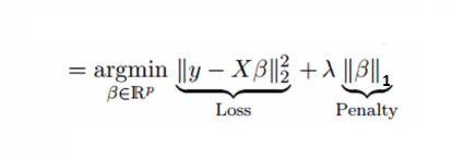
Where:
- λ (lambda) is the regularization parameter that controls the strength of the penalty. Higher values of λ lead to stronger regularization and more coefficients being pushed towards zero.
- βi is the coefficient associated with the i-th predictor.
The L1 penalty has a unique property that it promotes sparsity. This means that it encourages some coefficients to be exactly zero, effectively performing feature selection. In contrast to the L2 penalty (Ridge penalty), which squares the coefficients and promotes small but non-zero values, the L1 penalty tends to lead to sparse solutions where only a subset of predictors are chosen. As a result, the LASSO automatically performs feature selection, which is especially advantageous when dealing with high-dimensional datasets where many predictors may have negligible effects on the outcome.
Compare full-dim and LASSO results
Load full dim, zscored, data
We’ll use most of the data for the test set so that this dataset’s dimensionality begins to approach the number of observations. Regularization techniques such as LASSO tend to shine when working in this context. If you have plenty of data to estimate each coefficient, you will typically find that an unregularized model performs better.
from preprocessing import prep_fulldim_zdata
X_train_z, X_holdout_z, y_train, y_holdout, y = prep_fulldim_zdata(const_thresh= 95, test_size=.95, y_log_scaled=True)

from sklearn.model_selection import train_test_split
X_val_z, X_test_z, y_val, y_test = train_test_split(X_holdout_z, y_holdout, test_size=0.5, random_state=0)
X_train_z.head()
133 columns removed, 82 remaining.
Columns removed: ['MasVnrArea', 'LowQualFinSF', 'GarageYrBlt', '3SsnPorch', 'LotFrontage', 'KitchenAbvGr', 'PoolArea', 'Condition1_Artery', 'Condition1_PosA', 'Condition1_PosN', 'Condition1_RRAe', 'Condition1_RRAn', 'Condition1_RRNe', 'Condition1_RRNn', "Exterior2nd_'Brk Cmn'", "Exterior2nd_'Wd Shng'", 'Exterior2nd_AsbShng', 'Exterior2nd_AsphShn', 'Exterior2nd_BrkFace', 'Exterior2nd_CBlock', 'Exterior2nd_CmentBd', 'Exterior2nd_ImStucc', 'Exterior2nd_Other', 'Exterior2nd_Stone', 'Exterior2nd_Stucco', 'LotConfig_FR2', 'LotConfig_FR3', 'Alley_Grvl', 'Alley_Pave', 'RoofMatl_ClyTile', 'RoofMatl_CompShg', 'RoofMatl_Membran', 'RoofMatl_Metal', 'RoofMatl_Roll', 'RoofMatl_Tar&Grv', 'RoofMatl_WdShake', 'RoofMatl_WdShngl', 'Heating_Floor', 'Heating_GasA', 'Heating_GasW', 'Heating_Grav', 'Heating_OthW', 'Heating_Wall', 'MasVnrType_BrkCmn', 'Condition2_Artery', 'Condition2_Feedr', 'Condition2_Norm', 'Condition2_PosA', 'Condition2_PosN', 'Condition2_RRAe', 'Condition2_RRAn', 'Condition2_RRNn', 'HouseStyle_1.5Unf', 'HouseStyle_2.5Fin', 'HouseStyle_2.5Unf', 'HouseStyle_SFoyer', 'HouseStyle_SLvl', 'GarageType_2Types', 'GarageType_Basment', 'GarageType_CarPort', "MSZoning_'C (all)'", 'MSZoning_FV', 'MSZoning_RH', 'RoofStyle_Flat', 'RoofStyle_Gambrel', 'RoofStyle_Mansard', 'RoofStyle_Shed', 'Utilities_AllPub', 'Utilities_NoSeWa', 'SaleCondition_AdjLand', 'SaleCondition_Alloca', 'SaleCondition_Family', 'Neighborhood_Blmngtn', 'Neighborhood_Blueste', 'Neighborhood_BrDale', 'Neighborhood_BrkSide', 'Neighborhood_ClearCr', 'Neighborhood_Crawfor', 'Neighborhood_IDOTRR', 'Neighborhood_MeadowV', 'Neighborhood_Mitchel', 'Neighborhood_NPkVill', 'Neighborhood_NoRidge', 'Neighborhood_SWISU', 'Neighborhood_SawyerW', 'Neighborhood_StoneBr', 'Neighborhood_Timber', 'Neighborhood_Veenker', 'MiscFeature_Gar2', 'MiscFeature_Othr', 'MiscFeature_Shed', 'MiscFeature_TenC', 'BldgType_2fmCon', 'BldgType_Duplex', 'BldgType_Twnhs', 'SaleType_COD', 'SaleType_CWD', 'SaleType_Con', 'SaleType_ConLD', 'SaleType_ConLI', 'SaleType_ConLw', 'SaleType_Oth', 'Foundation_Slab', 'Foundation_Stone', 'Foundation_Wood', 'Electrical_FuseF', 'Electrical_FuseP', 'Electrical_Mix', 'LandContour_Bnk', 'LandContour_HLS', 'LandContour_Low', 'MSSubClass_30', 'MSSubClass_40', 'MSSubClass_45', 'MSSubClass_70', 'MSSubClass_75', 'MSSubClass_80', 'MSSubClass_85', 'MSSubClass_90', 'MSSubClass_160', 'MSSubClass_180', 'MSSubClass_190', 'Exterior1st_AsbShng', 'Exterior1st_AsphShn', 'Exterior1st_BrkComm', 'Exterior1st_BrkFace', 'Exterior1st_CBlock', 'Exterior1st_CemntBd', 'Exterior1st_ImStucc', 'Exterior1st_Stone', 'Exterior1st_Stucco', 'Exterior1st_WdShing', 'Street']
| BsmtFinSF1 | GarageCars | 1stFlrSF | YrSold | EnclosedPorch | WoodDeckSF | 2ndFlrSF | OpenPorchSF | BsmtHalfBath | GrLivArea | ... | MSSubClass_20 | MSSubClass_50 | MSSubClass_60 | MSSubClass_120 | Exterior1st_'Wd Sdng' | Exterior1st_HdBoard | Exterior1st_MetalSd | Exterior1st_Plywood | Exterior1st_VinylSd | CentralAir | |
|---|---|---|---|---|---|---|---|---|---|---|---|---|---|---|---|---|---|---|---|---|---|
| 633 | 0.075477 | -1.072050 | -0.173045 | -0.495091 | -0.251998 | 2.007070 | -0.849556 | -0.694796 | 4.124766 | -0.961978 | ... | 1.223298 | -0.117041 | -0.589094 | -0.239117 | 2.357786 | -0.372423 | -0.462275 | -0.323431 | -0.85322 | 0.166683 |
| 908 | -0.352031 | 0.350853 | -0.589792 | -1.203750 | -0.251998 | 0.434247 | -0.849556 | -0.694796 | -0.239117 | -1.313923 | ... | 1.223298 | -0.117041 | -0.589094 | -0.239117 | -0.418317 | 2.648339 | -0.462275 | -0.323431 | -0.85322 | 0.166683 |
| 611 | 0.374016 | 0.350853 | -0.237993 | -0.495091 | -0.251998 | -0.707093 | -0.849556 | -0.694796 | 4.124766 | -1.016827 | ... | -0.806264 | -0.117041 | -0.589094 | -0.239117 | -0.418317 | 2.648339 | -0.462275 | -0.323431 | -0.85322 | 0.166683 |
| 398 | -1.070913 | -1.072050 | -0.116216 | -0.495091 | -0.251998 | -0.707093 | -0.849556 | -0.694796 | -0.239117 | -0.913986 | ... | -0.806264 | -0.117041 | -0.589094 | -0.239117 | -0.418317 | -0.372423 | 2.133579 | -0.323431 | -0.85322 | 0.166683 |
| 91 | 0.362075 | 0.350853 | 0.311355 | -1.203750 | -0.251998 | -0.707093 | -0.849556 | -0.694796 | -0.239117 | -0.552900 | ... | 1.223298 | -0.117041 | -0.589094 | -0.239117 | -0.418317 | 2.648339 | -0.462275 | -0.323431 | -0.85322 | 0.166683 |
5 rows × 82 columns
print(X_train_z.shape)
(73, 82)
Intro to LassoCV
LassoCV in scikit-learn performs cross-validation to find the best alpha value (lambdas in traditional LASSO equation) from the specified list of alphas. It does this by fitting a separate LASSO regression for each alpha value on each fold of the cross-validation. The alphas parameter determines the values of alpha to be tested.
Cross-validation is a method used to assess the performance and generalizability of a machine learning model. It involves partitioning the dataset into multiple subsets, training the model on some of these subsets, and then evaluating its performance on the remaining subset(s).
For example, in 5-fold cross-validation, you split your data into 5 partitions (“folds”). You then train the model on 4 of the folds, leaving one out for validation. You do this 5 times — training/validating on different folds each time.
The LassoCV() functions returns the best model that was determined based on cross-validation performance. This best model’s coefficients can be accessed using the .coef_ attribute, and the optimal alpha can be accessed using the .alpha_ attribute.
from sklearn.linear_model import LassoCV
# help(LassoCV)
Specify range of alphas to evaluate
Specify a range of alpha values. Typically, small alphas work well. However, you don’t want to be so close to zero that you get no benefits from regularization (i.e., none of the coefs shrink to zero).
import numpy as np
alphas = np.logspace(-4, 1, 100) # The alphas you want to evaluate during cross-validation
alphas_with_zero = np.insert(alphas, 0, 0) # The unregularized model
print(alphas_with_zero[0:10])
max_iter = 100000 # This is the maximum number of iterations for which we want the model to run if it doesn’t converge before reaching this number. The default value is 1000
cv = 5 # number of folds to use during cross-validation
[0. 0.0001 0.00011233 0.00012619 0.00014175 0.00015923
0.00017886 0.00020092 0.0002257 0.00025354]
Call LassoCV
lasso_cv = LassoCV(alphas=alphas, cv=cv, max_iter=max_iter, random_state=0)
Randomness in LassoCV
LassoCV uses coordinate descent, which is a convex optimization algorithm meaning that it solves for a global optimum (one possible optimum).
However, during coordinate descent, when multiple features are highly correlated, the algorithm can choose any one of them to update at each iteration. This can lead to some randomness in the selection of features and the order in which they are updated. While coordinate descent itself is deterministic, the order in which the correlated features are selected can introduce variability.
The random state argument in LassoCV allows you to control this randomness by setting a specific random seed. This can be helpful for reproducibility when working with models that involve correlated features. By specifying a random seed, you ensure that the same features will be chosen in the same order across different runs of the algorithm, making the results more predictable and reproducible.
In summary, while coordinate descent is a convex algorithm, the random state argument in LassoCV helps manage the potential randomness introduced by the selection of correlated features during the optimization process.
# fit the model
best_lasso_model = lasso_cv.fit(X_train_z, y_train)
Print the best alpha value selected.
best_lasso_model.alpha_
0.0093260334688322
Print the coefs
coefs = best_lasso_model.coef_
coefs
array([ 0. , 0.06596183, 0. , -0. , 0.00999046,
0.02956164, 0. , 0.02594706, 0. , 0.08300968,
-0. , 0.03157657, 0.06126806, 0.01329162, 0.03171758,
-0.01378301, 0. , 0. , 0. , 0.04026495,
-0. , 0.0609676 , 0. , 0.00054206, 0.00410852,
0.00141018, 0. , -0. , 0.01709261, -0. ,
-0. , 0. , 0.00041337, 0.02716718, 0. ,
0. , -0. , 0.00381712, -0. , -0. ,
0. , -0. , -0. , 0. , -0. ,
0. , 0. , -0.04891258, 0.00014635, -0. ,
-0.02633333, 0. , 0. , 0. , -0. ,
-0. , -0. , 0. , 0.02453974, 0.02236798,
-0.02465517, 0. , 0. , 0.00378062, 0. ,
0. , -0.00136852, 0. , 0.00914042, -0. ,
0. , -0. , 0. , 0. , 0. ,
0. , -0.00601784, -0. , 0. , 0. ,
0. , 0.01252988])
Assess sparsity
percent_sparsity = np.mean(coefs == 0) * 100
percent_sparsity
63.41463414634146
Evaluate model error
from regression_predict_sklearn import measure_model_err
# to calculate residuals and R-squared for the test set, we'll need to get the model predictions first
y_pred_train = best_lasso_model.predict(X_train_z)
y_pred_test = best_lasso_model.predict(X_test_z)
errors_df = measure_model_err(y, np.mean(y),
y_train, y_pred_train,
y_test, y_pred_test,
'RMSE', y_log_scaled=True)
errors_df.head()
| Baseline Error | Train Error | Test Error | |
|---|---|---|---|
| 0 | 79415.291886 | 13763.876079 | 56009.758064 |
Use fit_eval_model() to quickly compare models
from regression_predict_sklearn import fit_eval_model
# Full-dim model
fulldim_model, error_df = fit_eval_model(y=y, baseline_pred=y.mean(),
X_train=X_train_z, y_train=y_train,
X_test=X_test_z, y_test=y_test,
predictors=X_train_z.columns,
metric='RMSE',
y_log_scaled=True,
model_type='unregularized',
include_plots=True, plot_raw=True, verbose=True)
# LASSO
import numpy as np
best_lasso_model, error_df = fit_eval_model(y=y, baseline_pred=y.mean(),
X_train=X_train_z, y_train=y_train,
X_test=X_test_z, y_test=y_test,
predictors=X_train_z.columns,
metric='RMSE',
y_log_scaled=True,
model_type='LassoCV', alphas=alphas, cv=cv, max_iter=max_iter,
include_plots=True, plot_raw=True, verbose=True)
# of predictor vars = 82
# of train observations = 73
# of test observations = 694
Baseline RMSE = 79415.29188606751
Train RMSE = 2.905594915676157e-10
Holdout RMSE = 2357924.397903089
(Holdout-Train)/Train: 811511744180753792%
# of predictor vars = 82
# of train observations = 73
# of test observations = 694
Baseline RMSE = 79415.29188606751
Train RMSE = 13763.876078966621
Holdout RMSE = 56009.758063855006
(Holdout-Train)/Train: 307%
Investivating the alpha hyperparameter
Here, we will take a closer look at the alpha hyperparameter to see which values performed well.
We will see different values of alpha impact:
- train error
- validation error
- coefficient sparsity
Unfortunately for us, the LassoCV function in scikit-learn doesn’t store the train errors for each model evaluated. It’s primarily designed to perform cross-validation to find the best alpha value for Lasso regression regularization. For our purposes, we will have to manually run Lasso for each alpha value.
Typically when comparing alpha values, you’re in the model selection stage of your analysis. This means that you need to use the validation set to evaluate performance. LassoCV does this implicitly by using portions of the training data as validation data. Here, we’ll use the explicit validation set we defined at the beginning of this episode.
import matplotlib.pyplot as plt
# Calculate the corresponding training scores for each alpha and fold
from sklearn.linear_model import Lasso
train_scores = []
val_scores = []
perc_sparse_vals = []
for alpha in alphas:
lasso = Lasso(alpha=alpha, max_iter=max_iter)
lasso.fit(X_train_z, y_train)
coefs = lasso.coef_
percent_sparse = np.mean(coefs == 0) * 100
train_pred = lasso.predict(X_train_z)
val_pred = lasso.predict(X_val_z)
train_scores.append(np.mean((train_pred - y_train) ** 2))
val_scores.append(np.mean((val_pred - y_val) ** 2))
perc_sparse_vals.append(percent_sparse)
# Create a grid of subplots
fig, (ax1, ax2) = plt.subplots(1, 2, figsize=(12, 5))
# Plot the training and validation scores
ax1.plot(np.log10(alphas), train_scores, label='Train', marker='o')
ax1.plot(np.log10(alphas), val_scores, label='Validation (CV)', marker='o')
ax1.set_xlabel('log(alpha)')
ax1.set_ylabel('Mean Squared Error')
ax1.set_title('LassoCV Train/Validation Scores')
ax1.legend()
ax1.grid(True)
# Plot percent sparsity
ax2.plot(np.log10(alphas), perc_sparse_vals, label='Percent Sparsity', marker='o', color='orange')
ax2.set_xlabel('log(alpha)')
ax2.set_ylabel('Percent Sparsity')
ax2.set_title('Percent Sparsity vs. alpha')
ax2.grid(True)
# Adjust layout and display the plots
plt.tight_layout()
plt.savefig('..//fig//regression//regularize//alpha_cv_results.png', bbox_inches='tight', dpi=300, facecolor='white');

LASSO as a feature selection method
A well optimized LASSO model can be used as a data-driven feature selection method. However, one thing to be mindful of is, given two features that are correlated, LASSO may randomly select one feature’s coefficient to shrink to zero. This can sometimes lead to less desirable model specifications. However, if you have one are more features that you want to ensure are included in the model, you can follow this procedure:
- Fit the LassoCV model to determine the optimal features to keep in the model,
feats_keep - Extend the list of
feats_keepto include other features/predictors that are important to your research questions - Fit a standard unregularized model using
feats_keepas your predictors - Take care to check the assumptions of the model, especially if you’re adding features after selecting them with LASSO. LASSO helps prevent multicollinearity issues, but adding features back in could re-introduce multicollinearity
Let’s see which features our best LASSO model decided to keep.
from interpret_model import coef_plot
# Get coefficient matrix
coef_matrix = best_lasso_model.coef_
fig = coef_plot(coefs=coef_matrix, plot_const=False, index=X_train_z.columns)
fig.set_size_inches(6, 8)
Introduction to the ridge model in high-dimensional data analysis
Ridge regression introduces an L2 penalty term to the linear regression equation, which involves adding the squared magnitudes of the coefficients to the loss function. This regularization technique aims to minimize the sum of squared residuals while also constraining the coefficients. Here are some key points about Ridge regression:
-
Coefficient Shrinkage: Ridge regression shrinks the coefficients towards zero by penalizing their magnitudes. However, unlike Lasso, Ridge regression does not force any coefficients to become exactly zero.
-
Multicollinearity Mitigation: Both Ridge and Lasso provide ways to handle multicollinearity, but their mechanisms and outcomes are somewhat different. Ridge regression provides a more continuous shrinkage of coefficients, while Lasso can lead to sparse models with only a subset of predictors retained.
-
Inclusion of All Predictors: Ridge regression retains all predictors in the model, even if some predictors have relatively small coefficients. This can be beneficial when you believe that most predictors contribute to the outcome, but you want to reduce their impact to avoid overfitting.
-
Bias-Variance Trade-off (avoids overfitting): Ridge regression strikes a balance between bias and variance. It can reduce the risk of overfitting without excluding any predictors from the model, making it a useful tool when working with high-dimensional datasets.
In summary, Ridge regression and Lasso are regularization techniques that address high-dimensional data analysis challenges in distinct ways. Ridge regression is effective for shrinking coefficients to small values, but keeping all predictors in the model. Lasso excels in situations where feature selection and interpretability are essential. The choice between Ridge regression and Lasso depends on the specific goals of your analysis and the nature of your dataset.
The L2 penalty
The fundamental principle underlying ridge regression is its utilization of the L2 penalty, which involves the summation of the squared values of the coefficients (parameters) of the model, multiplied by a regularization parameter (often represented as λ or alpha).
In the realm of linear regression, the L2 penalty can be integrated into the ordinary least squares (OLS) loss function in the following manner:
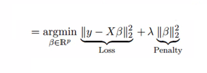
from sklearn.linear_model import LinearRegression, RidgeCV
ridge_cv = RidgeCV(alphas=alphas, store_cv_values=True) # store_cv_values=True to enable cv_values_
# Fit the RidgeCV model
ridge_cv.fit(X_train_z, y_train)
# Print the chosen alpha and corresponding R-squared score
print("Chosen Alpha:", ridge_cv.alpha_)
print("R-squared Score:", ridge_cv.score(X_test_z, y_test))
Chosen Alpha: 10.0
R-squared Score: 0.8108420609911078
# Full-dimensional linear regression
full_dim_model = LinearRegression()
full_dim_model.fit(X_train_z, y_train)
full_dim_r2 = full_dim_model.score(X_test_z, y_test)
print("R-squared Score:", full_dim_r2)
R-squared Score: -7.321193011831792
from interpret_model import coef_plot
# Get coefficient matrix
coef_matrix = ridge_cv.coef_
fig = coef_plot(coefs=coef_matrix, plot_const=False, index=X_train_z.columns)
fig.set_size_inches(6, 15)
Elastic Net
Elastic Net is a regularization technique used in linear regression models that combines both L1 (LASSO) and L2 (ridge) penalties. It aims to address some limitations of individual LASSO and ridge regression by providing a balance between feature selection (LASSO’s sparsity) and coefficient shrinkage (ridge’s stability).
The Elastic Net regularization term can be represented as a combination of the L1 and L2 penalties, and it depends on two hyperparameters: α (alpha) and λ (lambda). The α parameter controls the balance between the L1 and L2 penalties. When α is 0, Elastic Net behaves like ridge regression, and when α is 1, it behaves like LASSO.
To implement Elastic Net in Python, you can use libraries like scikit-learn. Here’s how you can do it:
# Initialize the ElasticNetCV model
alphas = [0.1, 1.0, 10.0] # List of alpha values to search over
l1_ratios = [0.1, 0.5, 0.9] # List of l1_ratio values to search over
elastic_net_cv = ElasticNetCV(alphas=alphas, l1_ratio=l1_ratios, cv=5)
Key Points
Exploring additional datasets
Overview
Teaching: 45 min
Exercises: 2 minQuestions
How can we use everything we have learned to analyze a new dataset?
Objectives
Preprocessing
Note: Adapt get_feat_types() and encode_predictors_housing_data() for your data. Use new functions with slightly different names.
# get geat types - you'll need to create a similar function for your data that stores the type of each predictor
from preprocessing import get_feat_types
predictor_type_dict = get_feat_types()
continuous_fields = predictor_type_dict['continuous_fields']
# encode predictors (one-hot encoding for categorical data) - note you may have to create a new function starting from a copy of this one
from preprocessing import encode_predictors_housing_data
X_encoded = encode_predictors_housing_data(X)
# remove columns with nans or containing > 95% constant values (typically 0's)
from preprocessing import remove_bad_cols
X_good = remove_bad_cols(X, 95)
# train/test splits
from sklearn.model_selection import train_test_split
x_train, x_test, y_train, y_test = train_test_split(x, y_log,
test_size=0.33,
random_state=0)
print(x_train.shape)
print(x_test.shape)
# zscore
from preprocessing import zscore
# get means and stds
train_means = X_train.mean()
train_stds = X_train.std()
X_train_z = zscore(df=X_train, train_means=train_means, train_stds=train_stds)
X_test_z = zscore(df=X_test, train_means=train_means, train_stds=train_stds)
X_train_z.head()
# get random predictor permutations...
from preprocessing import get_predictor_combos
sampled_combinations = get_predictor_combos(X_train=X_train, K=K, n=25)
Feature selection
from feature_selection import get_best_uni_predictors
top_features = get_best_uni_predictors(N_keep=5, y=y, baseline_pred=y.mean(),
X_train=X_train, y_train=y_train,
X_val=X_val, y_val=y_val,
metric='RMSE', y_log_scaled=True)
top_features
Fit/eval model (sklearn version)
from regression_predict_sklearn import fit_eval_model
fit_eval_model(y=y, baseline_pred=y.mean(),
X_train=X_train_z, y_train=y_train,
X_test=X_test_z, y_test=y_test,
predictors=X_train_z.columns,
metric='RMSE',
y_log_scaled=True,
model_type='unregularized',
include_plots=True, plot_raw=True, verbose=True)
Model eval
# plot (1) true vs predicted vals for train/test sets and (2) best line of fit (only applies for univariate models)
from regression_predict_sklearn import plot_train_test_predictions
(fig1, fig2) = plot_train_test_predictions(predictors=[predictor],
X_train=x_train, X_test=x_test,
y_train=y_train, y_test=y_test,
y_pred_train=y_pred_train, y_pred_test=y_pred_test,
y_log_scaled=True, plot_raw=True);
# report baseline, train, and test errors
from regression_predict_sklearn import measure_model_err
error_df = measure_model_err(y=y, baseline_pred=baseline_predict,
y_train=y_train, y_pred_train=y_pred_train,
y_test=y_test, y_pred_test=y_pred_test,
metric='MAPE', y_log_scaled=False)
error_df.head()
Comparing models…
df_model_err = compare_models(y=y, baseline_pred=baseline_predict,
X_train=X_train, y_train=y_train,
X_val=X_val, y_val=y_val,
predictors_list=X_train.columns,
metric='RMSE', y_log_scaled=True,
model_type='unregularized',
include_plots=False, plot_raw=False, verbose=False)
Key Points
Clustering high dimensional data
Overview
Teaching: 45 min
Exercises: minQuestions
TODO
Objectives
TODO
Key Points
TODO
Data visualization techniques: t-SNE and PaCMAP
Overview
Teaching: 45 min
Exercises: minQuestions
TODO
Objectives
TODO
Key Points
TODO