Manipulating, analyzing and exporting data with tidyverse
Overview
Teaching: min
Exercises: minQuestions
Objectives
Describe the purpose of the
dplyrandtidyrpackages.Select certain columns in a data frame with the
dplyrfunctionselect.Select certain rows in a data frame according to filtering conditions with the
dplyrfunctionfilter.Link the output of one
dplyrfunction to the input of another function with the ‘pipe’ operator%>%.Add new columns to a data frame that are functions of existing columns with
mutate.Use the split-apply-combine concept for data analysis.
Use
summarize,group_by, andcountto split a data frame into groups of observations, apply summary statistics for each group, and then combine the results.Describe the concept of a wide and a long table format and for which purpose those formats are useful.
Reshape a data frame from long to wide format and back with the
pivot_widerandpivot_longercommands from thetidyrpackage.Export a data frame to a .csv file.
Manipulating and analyzing data with dplyr
Data Manipulation using dplyr and tidyr
Bracket subsetting is handy, but it can be cumbersome and difficult to read,
especially for complicated operations. Enter dplyr. dplyr is a package for
making tabular data manipulation easier. It pairs nicely with tidyr which enables you to swiftly convert between different data formats for plotting and analysis.
Packages in R are basically sets of additional functions that let you do more
stuff. The functions we’ve been using so far, like str() or data.frame(),
come built into R; packages give you access to more of them. Before you use a
package for the first time you need to install it on your machine, and then you
should import it in every subsequent R session when you need it. You should
already have installed the tidyverse package. This is an
“umbrella-package” that installs several packages useful for data analysis which
work together well such as tidyr, dplyr, ggplot2, tibble, etc.
The tidyverse package tries to address 3 common issues that arise when
doing data analysis with some of the functions that come with R:
- The results from a base R function sometimes depend on the type of data.
- Using R expressions in a non standard way, which can be confusing for new learners.
- Hidden arguments, having default operations that new learners are not aware of.
We have seen in our previous lesson that when building or importing a data frame, the columns that contain characters (i.e., text) are coerced (=converted) into the factor data type. We had to set stringsAsFactors to FALSE to avoid this hidden argument to convert our data type.
This time we will use the tidyverse package to read the data and avoid having to set stringsAsFactors to FALSE
To load the package type:
## load the tidyverse packages, incl. dplyr
library("tidyverse")
What are dplyr and tidyr?
The package dplyr provides easy tools for the most common data manipulation
tasks. It is built to work directly with data frames, with many common tasks
optimized by being written in a compiled language (C++). An additional feature is the
ability to work directly with data stored in an external database. The benefits of
doing this are that the data can be managed natively in a relational database,
queries can be conducted on that database, and only the results of the query are
returned.
This addresses a common problem with R in that all operations are conducted in-memory and thus the amount of data you can work with is limited by available memory. The database connections essentially remove that limitation in that you can connect to a database of many hundreds of GB, conduct queries on it directly, and pull back into R only what you need for analysis.
The package tidyr addresses the common problem of wanting to reshape your data for plotting and use by different R functions. Sometimes we want data sets where we have one row per measurement. Sometimes we want a data frame where each measurement type has its own column, and rows are instead more aggregated groups - like plots or aquaria. Moving back and forth between these formats is nontrivial, and tidyr gives you tools for this and more sophisticated data manipulation.
To learn more about dplyr and tidyr after the workshop, you may want to check out this
handy data transformation with dplyr cheatsheet and this one about tidyr.
We’ll read in our data using the read_csv() function, from the tidyverse package readr, instead of read.csv().
adni_r <- read_csv("data/ADNIMERGE.csv")

## inspect the data
str(adni_r)
## preview the data
View(adni_r)
Notice that the class of the data is now tbl_df
This is referred to as a “tibble”. Tibbles tweak some of the behaviors of the data frame objects we introduced in the previous episode. The data structure is very similar to a data frame. For our purposes the only differences are that:
- In addition to displaying the data type of each column under its name, it only prints the first few rows of data and only as many columns as fit on one screen.
- Columns of class
characterare never converted into factors.
Missing data
You may notice that many of the fields have the value -4. This number is the code for missing data in the ADNI dataset. To read these in as missing data, denoted by NA in the R programming language, we can use the na argument to the read_csv() function to specify that these values are missing.
adni_r <- read_csv("data/ADNIMERGE.csv",
                 na = "-4")

View(adni_r)
dplyr
We’re going to learn some of the most common dplyr functions:
select(): subset columnsfilter(): subset rows on conditionsmutate(): create new columns by using information from other columnsgroup_by()andsummarize(): create summary statistics on grouped dataarrange(): sort resultscount(): count discrete values
Selecting columns and filtering rows
To select columns of a data frame, use select(). The first argument
to this function is the data frame (adni_r), and the subsequent
arguments are the columns to keep.
select(adni_r, PTID, EXAMDATE_mod, DX)
To select all columns except certain ones, put a “-“ in front of the variable to exclude it.
select(adni_r, -PTID, -DX)
This will select all the variables in adni_r except RID
and DX.
To choose rows based on a specific criteria, use filter():
filter(adni_r, AGE_mod < 60)
# A tibble: 432 x 14
   PTID  VISCODE AGE_mod PTGENDER PTMARRY PTEDUCAT DX     SITE EXAMDATE_mod
   <chr> <chr>     <dbl> <chr>    <chr>      <dbl> <chr> <dbl> <date>
 1 032_… bl         59.7 Female   Married       18 Deme…    32 2006-02-22
 2 032_… m06        59.7 Female   Married       18 Deme…    32 2006-08-30
 3 032_… m12        59.7 Female   Married       18 Deme…    32 2007-01-15
 4 032_… m24        59.7 Female   Married       18 Deme…    32 2008-03-24
 5 136_… bl         56.4 Male     Married       16 Deme…   136 2006-06-10
 6 136_… m06        56.4 Male     Married       16 Deme…   136 2006-10-28
 7 136_… m12        56.4 Male     Married       16 Deme…   136 2007-05-26
 8 136_… m24        56.4 Male     Married       16 Deme…   136 2008-04-29
 9 137_… bl         56.5 Female   Divorc…       20 Deme…   137 2006-05-18
10 137_… m06        56.5 Female   Divorc…       20 Deme…   137 2006-12-13
# … with 422 more rows, and 5 more variables: WholeBrain <dbl>,
#   WholeBrain_bl <dbl>, Hippocampus <dbl>, APOE4 <dbl>, TAU_mod <dbl>
Pipes
What if you want to select and filter at the same time? There are three ways to do this: use intermediate steps, nested functions, or pipes.
With intermediate steps, you create a temporary data frame and use that as input to the next function, like this:
adni_r2 <- filter(adni_r, AGE_mod < 60)
adni_r_young <- select(adni_r2, PTID, PTGENDER, AGE_mod)
This is readable, but can clutter up your workspace with lots of objects that you have to name individually. With multiple steps, that can be hard to keep track of.
You can also nest functions (i.e. one function inside of another), like this:
adni_r_young <- select(filter(adni_r, AGE_mod < 60), PTID, PTGENDER, AGE_mod)
This is handy, but can be difficult to read if too many functions are nested, as R evaluates the expression from the inside out (in this case, filtering, then selecting).
The last option, pipes, are a recent addition to R. Pipes let you take
the output of one function and send it directly to the next, which is useful
when you need to do many things to the same dataset. Pipes in R look like
%>% and are made available via the magrittr package, installed automatically
with dplyr. If you use RStudio, you can type the pipe with Ctrl
- Shift + M if you have a PC or Cmd + Shift + M if you have a Mac.
adni_r %>%
  filter(AGE_mod < 60) %>%
  select(PTID, PTGENDER, AGE_mod)
# A tibble: 432 x 3
   PTID       PTGENDER AGE_mod
   <chr>      <chr>      <dbl>
 1 032_S_0147 Female      59.7
 2 032_S_0147 Female      59.7
 3 032_S_0147 Female      59.7
 4 032_S_0147 Female      59.7
 5 136_S_0300 Male        56.4
 6 136_S_0300 Male        56.4
 7 136_S_0300 Male        56.4
 8 136_S_0300 Male        56.4
 9 137_S_0366 Female      56.5
10 137_S_0366 Female      56.5
# … with 422 more rows
In the above code, we use the pipe to send the adni_r dataset first through
filter() to keep rows where AGE_mod is less than 5, then through select()
to keep only the PTID, PTGENDER, and AGE_mod columns. Since %>% takes
the object on its left and passes it as the first argument to the function on
its right, we don’t need to explicitly include the data frame as an argument
to the filter() and select() functions any more.
Some may find it helpful to read the pipe like the word “then”. For instance,
in the above example, we took the data frame adni_r, then we filtered
for rows with AGE_mod < 60, then we selected columns PTID, VISCODE, PTGENDER,
and AGE_mod. The dplyr functions by themselves are somewhat simple,
but by combining them into linear workflows with the pipe, we can accomplish
more complex manipulations of data frames.
If we want to create a new object with this smaller version of the data, we can assign it a new name:
adni_r_young <- adni_r %>%
  filter(AGE_mod < 60) %>%
  select(PTID, PTGENDER, AGE_mod)

adni_r_young
# A tibble: 432 x 3
   PTID       PTGENDER AGE_mod
   <chr>      <chr>      <dbl>
 1 032_S_0147 Female      59.7
 2 032_S_0147 Female      59.7
 3 032_S_0147 Female      59.7
 4 032_S_0147 Female      59.7
 5 136_S_0300 Male        56.4
 6 136_S_0300 Male        56.4
 7 136_S_0300 Male        56.4
 8 136_S_0300 Male        56.4
 9 137_S_0366 Female      56.5
10 137_S_0366 Female      56.5
# … with 422 more rows
Note that the final data frame is the leftmost part of this expression.
Challenge
Using pipes, subset the
adni_rdata to include patients seen before 2008 and retain only the columnsEXAMDATE_mod,PTGENDER, andAGE_mod.Solution
adni_r %>%
    filter(EXAMDATE_mod < 2008-01-01) %>%
    select(EXAMDATE_mod, PTGENDER, AGE_mod)
Mutate
Frequently you’ll want to create new columns based on the values in existing
columns, for example to do unit conversions, or to find the ratio of values in two
columns. For this we’ll use mutate().
To create a new column that contains the year of the visit only using mutate and the lubridate package:
library(lubridate)

adni_r<-adni_r %>%
  mutate(year = year(EXAMDATE_mod))

adni_r
# A tibble: 13,900 x 15
   PTID  VISCODE AGE_mod PTGENDER PTMARRY PTEDUCAT DX     SITE EXAMDATE_mod
   <chr> <chr>     <dbl> <chr>    <chr>      <dbl> <chr> <dbl> <date>
 1 011_… bl         74.3 Male     Married       16 CN       11 2005-08-18
 2 011_… bl         81.3 Male     Married       18 Deme…    11 2005-10-11
 3 011_… m06        81.3 Male     Married       18 Deme…    11 2006-03-11
 4 011_… m12        81.3 Male     Married       18 Deme…    11 2006-09-29
 5 011_… m24        81.3 Male     Married       18 Deme…    11 2007-09-06
 6 022_… bl         67.5 Male     Married       10 MCI      22 2005-11-10
 7 022_… m06        67.5 Male     Married       10 MCI      22 2006-04-14
 8 022_… m12        67.5 Male     Married       10 MCI      22 2006-10-26
 9 022_… m18        67.5 Male     Married       10 MCI      22 2007-05-31
10 022_… m36        67.5 Male     Married       10 MCI      22 2008-10-30
# … with 13,890 more rows, and 6 more variables: WholeBrain <dbl>,
#   WholeBrain_bl <dbl>, Hippocampus <dbl>, APOE4 <dbl>, TAU_mod <dbl>,
#   year <dbl>
You can also create a second new column within the same call of mutate():
adni_r<-adni_r %>%
  mutate(year = year(EXAMDATE_mod),
         month = month(EXAMDATE_mod))


adni_r
# A tibble: 13,900 x 16
   PTID  VISCODE AGE_mod PTGENDER PTMARRY PTEDUCAT DX     SITE EXAMDATE_mod
   <chr> <chr>     <dbl> <chr>    <chr>      <dbl> <chr> <dbl> <date>
 1 011_… bl         74.3 Male     Married       16 CN       11 2005-08-18
 2 011_… bl         81.3 Male     Married       18 Deme…    11 2005-10-11
 3 011_… m06        81.3 Male     Married       18 Deme…    11 2006-03-11
 4 011_… m12        81.3 Male     Married       18 Deme…    11 2006-09-29
 5 011_… m24        81.3 Male     Married       18 Deme…    11 2007-09-06
 6 022_… bl         67.5 Male     Married       10 MCI      22 2005-11-10
 7 022_… m06        67.5 Male     Married       10 MCI      22 2006-04-14
 8 022_… m12        67.5 Male     Married       10 MCI      22 2006-10-26
 9 022_… m18        67.5 Male     Married       10 MCI      22 2007-05-31
10 022_… m36        67.5 Male     Married       10 MCI      22 2008-10-30
# … with 13,890 more rows, and 7 more variables: WholeBrain <dbl>,
#   WholeBrain_bl <dbl>, Hippocampus <dbl>, APOE4 <dbl>, TAU_mod <dbl>,
#   year <dbl>, month <dbl>
Challenge
Create a new data frame from the
adni_rdata that meets the following criteria: contains only theDXcolumn and a new column calleddaycontaining the day value from theEXAMDATE_modvariable. Keep only values from January of 2009Hint: think about how the commands should be ordered to produce this data frame!
Solution
  adni_r_day <- adni_r %>%
  mutate(day = (day(EXAMDATE_mod))) %>%
  filter(month == 1, year == 2009)%>%
  select(DX, day)
Split-apply-combine data analysis and the summarize() function
Many data analysis tasks can be approached using the split-apply-combine
paradigm: split the data into groups, apply some analysis to each group, and
then combine the results. dplyr makes this very easy through the use of the
group_by() function.
The summarize() function
group_by() is often used together with summarize(), which collapses each
group into a single-row summary of that group. group_by() takes as arguments
the column names that contain the categorical variables for which you want
to calculate the summary statistics. So to compute the mean AGE by gender:
adni_r %>%
  group_by(PTGENDER) %>%
  summarize(mean_age = mean(AGE_mod))
# A tibble: 2 x 2
  PTGENDER mean_age
  <chr>       <dbl>
1 Female         NA
2 Male           NA
You may also have noticed that the output from these calls doesn’t run off the
screen anymore. It’s one of the advantages of tbl_df over data frame.
You can also group by multiple columns:
adni_r %>%
  group_by(PTGENDER, DX) %>%
  summarize(mean_age = mean(AGE_mod))
# A tibble: 8 x 3
# Groups:   PTGENDER [2]
  PTGENDER DX       mean_age
  <chr>    <chr>       <dbl>
1 Female   CN           NA
2 Female   Dementia     73.4
3 Female   MCI          72.1
4 Female   <NA>         73.1
5 Male     CN           74.2
6 Male     Dementia     75.1
7 Male     MCI          NA
8 Male     <NA>         74.4
When grouping both by PTGENDER and DX, the table contains a row for each gender/diagnosis combination.
You can see that some of the patients did not have a diagnosis listed. To remove this row from the table, filter out the NA values in the DX column
is.na() is a function that determines whether something is an NA. The !
symbol negates the result, so we’re asking for every row where DX is not an NA.
adni_r %>%
  filter(!is.na(DX)) %>%
  group_by(PTGENDER, DX) %>%
  summarize(mean_age = mean(AGE_mod))
# A tibble: 6 x 3
# Groups:   PTGENDER [2]
  PTGENDER DX       mean_age
  <chr>    <chr>       <dbl>
1 Female   CN           NA
2 Female   Dementia     73.4
3 Female   MCI          72.1
4 Male     CN           74.2
5 Male     Dementia     75.1
6 Male     MCI          NA
Here, again, the output from these calls doesn’t run off the screen
anymore. If you want to display more data, you can use the print() function
at the end of your chain with the argument n specifying the number of rows to
display:
adni_r %>%
  filter(!is.na(DX)) %>%
  group_by(PTGENDER, DX) %>%
  summarize(mean_age = mean(AGE_mod)) %>%
  print(n = 15)
# A tibble: 6 x 3
# Groups:   PTGENDER [2]
  PTGENDER DX       mean_age
  <chr>    <chr>       <dbl>
1 Female   CN           NA
2 Female   Dementia     73.4
3 Female   MCI          72.1
4 Male     CN           74.2
5 Male     Dementia     75.1
6 Male     MCI          NA
Once the data are grouped, you can also summarize multiple variables at the same time (and not necessarily on the same variable). For instance, we could add a column indicating the minimum age for each diagnosis for each gender:
adni_r %>%
  filter(!is.na(DX)) %>%
  group_by(PTGENDER, DX) %>%
  summarize(mean_age = mean(AGE_mod),
            min_age = min(AGE_mod))
# A tibble: 6 x 4
# Groups:   PTGENDER [2]
  PTGENDER DX       mean_age min_age
  <chr>    <chr>       <dbl>   <dbl>
1 Female   CN           NA      NA
2 Female   Dementia     73.4    55
3 Female   MCI          72.1    55
4 Male     CN           74.2    59.6
5 Male     Dementia     75.1    55.3
6 Male     MCI          NA      NA
It is sometimes useful to rearrange the result of a query to inspect the values. For instance, we can sort on min_age to put the younger patients first:
adni_r %>%
  filter(!is.na(DX)) %>%
  group_by(PTGENDER, DX) %>%
  summarize(mean_age = mean(AGE_mod),
            min_age = min(AGE_mod)) %>%
  arrange(min_age)
# A tibble: 6 x 4
# Groups:   PTGENDER [2]
  PTGENDER DX       mean_age min_age
  <chr>    <chr>       <dbl>   <dbl>
1 Female   Dementia     73.4    55
2 Female   MCI          72.1    55
3 Male     Dementia     75.1    55.3
4 Male     CN           74.2    59.6
5 Female   CN           NA      NA
6 Male     MCI          NA      NA
To sort in descending order, we need to add the desc() function. If we want to sort the results by decreasing order of mean age:
adni_r %>%
  filter(!is.na(DX)) %>%
  group_by(PTGENDER, DX) %>%
  summarize(mean_age = mean(AGE_mod),
            min_age = min(AGE_mod)) %>%
  arrange(desc(mean_age))
# A tibble: 6 x 4
# Groups:   PTGENDER [2]
  PTGENDER DX       mean_age min_age
  <chr>    <chr>       <dbl>   <dbl>
1 Male     Dementia     75.1    55.3
2 Male     CN           74.2    59.6
3 Female   Dementia     73.4    55
4 Female   MCI          72.1    55
5 Female   CN           NA      NA
6 Male     MCI          NA      NA
Counting
When working with data, we often want to know the number of observations found
for each factor or combination of factors. For this task, dplyr provides
count(). For example, if we wanted to count the number of rows of data for
each gender, we would do:
adni_r %>%
    count(PTGENDER)
# A tibble: 2 x 2
  PTGENDER     n
  <chr>    <int>
1 Female    6131
2 Male      7769
The count() function is shorthand for something we’ve already seen: grouping by a variable, and summarizing it by counting the number of observations in that group. In other words, adni_r %>% count(PTGENDER) is equivalent to:
adni_r %>%
    group_by(PTGENDER) %>%
    summarise(count = n())
# A tibble: 2 x 2
  PTGENDER count
  <chr>    <int>
1 Female    6131
2 Male      7769
For convenience, count() provides the sort argument:
adni_r %>%
    count(PTGENDER, sort = TRUE)
# A tibble: 2 x 2
  PTGENDER     n
  <chr>    <int>
1 Male      7769
2 Female    6131
Previous example shows the use of count() to count the number of rows/observations
for one factor (i.e., sex).
If we wanted to count combination of factors, such as PTGENDER and DX,
we would specify the first and the second factor as the arguments of count():
adni_r %>%
  count(PTGENDER, DX)
# A tibble: 8 x 3
  PTGENDER DX           n
  <chr>    <chr>    <int>
1 Female   CN        1697
2 Female   Dementia   950
3 Female   MCI       1725
4 Female   <NA>      1759
5 Male     CN        1584
6 Male     Dementia  1263
7 Male     MCI       2641
8 Male     <NA>      2281
With the above code, we can proceed with arrange() to sort the table
according to a number of criteria so that we have a better comparison.
For instance, we might want to arrange the table above in (i) an alphabetical order of
the levels of the species and (ii) in descending order of the count:
adni_r %>%
  count(PTGENDER, DX) %>%
  arrange(PTGENDER, desc(n))
# A tibble: 8 x 3
  PTGENDER DX           n
  <chr>    <chr>    <int>
1 Female   <NA>      1759
2 Female   MCI       1725
3 Female   CN        1697
4 Female   Dementia   950
5 Male     MCI       2641
6 Male     <NA>      2281
7 Male     CN        1584
8 Male     Dementia  1263
From the table above, we can see that there are 950 observations of women diagnosed with dementia.
Challenge
- How many visits were there at each
SITEin this study?Solution
adni_r %>%
   count(SITE)
# A tibble: 67 x 2 SITE n <dbl> <int> 1 2 367 2 3 278 3 5 209 4 6 194 5 7 254 6 9 195 7 10 98 8 11 295 9 12 203 10 13 171 # … with 57 more rows
- Use
group_by()andsummarize()to find the mean, min, and maxPTEDUCATfor each diagnosis (usingDX). Also add the number of observations (hint: see?n).Solution
adni_r %>%
    filter(!is.na(PTEDUCAT)) %>%
    group_by(DX) %>%
    summarize(
        mean_edu = mean(PTEDUCAT),
        min_edu = min(PTEDUCAT),
        max_edu = max(PTEDUCAT),
        n = n()
    )
# A tibble: 4 x 5 DX mean_edu min_edu max_edu n <chr> <dbl> <dbl> <dbl> <int> 1 CN 16.5 6 20 3281 2 Dementia 15.5 4 20 2213 3 MCI 16.0 4 20 4366 4 <NA> 16.1 6 20 4040
- What was the youngest patient seen at each site? Return the columns
year,DX, andage.Solution
adni_r %>%
    filter(!is.na(AGE_mod)) %>%
    group_by(SITE) %>%
    filter(AGE_mod == min(AGE_mod)) %>%
    select(year, DX, AGE_mod)
# A tibble: 343 x 4 # Groups: SITE [67] SITE year DX AGE_mod <dbl> <dbl> <chr> <dbl> 1 32 2006 Dementia 59.7 2 32 2006 Dementia 59.7 3 32 2007 Dementia 59.7 4 32 2008 Dementia 59.7 5 21 2006 MCI 60.3 6 21 2006 MCI 60.3 7 21 2007 MCI 60.3 8 21 2008 Dementia 60.3 9 21 2008 Dementia 60.3 10 136 2006 Dementia 56.4 # … with 333 more rows
Reshaping data with tidyr
In the spreadsheet lesson, we discussed how to structure our data leading to the four rules defining a tidy dataset:
- Each variable has its own column
- Each observation has its own row
- Each value must have its own cell
- Each type of observational unit forms a table
Here we examine the fourth rule: Each type of observational unit forms a table.
In the ADNI dataset , the rows of adni_r contain the values of variables associated
with each patient visit (the unit), values such the age or gender of each patient
associated with each visit. What if instead of comparing records, we wanted to compare the mean age of patients with the same diagnoses at different sites?
We’d need to create a new table where each row (the unit) is comprised of values of variables associated with each study site. In practical terms this means the values of diagnosis would become the names of column variables and the cells would contain the values of the mean age observed at each study site.
Having created a new table, we can explore the relationship between the age of patients with different diagnoses within, and between, the study sites. The key point here is that we are still following a tidy data structure, but we have reshaped the data according to the observations of interest: average age of patient with a certain diagnosis per study site instead of by patient visits.
The opposite transformation would be to transform column names into values of a variable.
We can do both these of transformations with two tidyr functions, pivot_longer()
and pivot_wider().
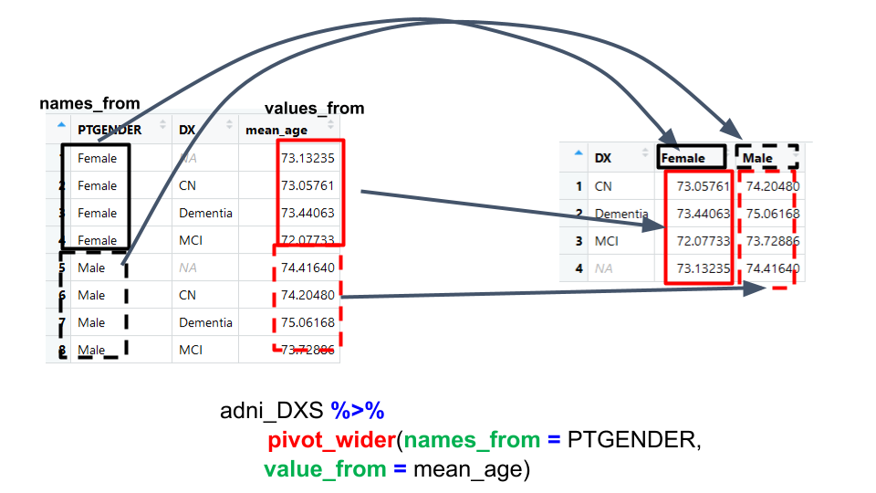
Creating wide data
pivot_wider() takes three principal arguments:
- the data to be reshaped (a dataframe)
- names_from - values will become new column names.
- values_from - values will fill the new column variables.
Further arguments include values_fill which, if set, fills in missing values with
the value provided.
Let’s use pivot_wider() to transform the dataset to find the mean age of female or male patients for each diagnosis over the entire study. We use filter(),
group_by() and summarise() to filter our observations and variables of
interest, and create a new variable for the mean_age. We use the pipe as
before too.
adni_r_DXS <- adni_r %>%
  filter(!is.na(AGE_mod)) %>%
  group_by(PTGENDER, DX) %>%
  summarize(mean_age = mean(AGE_mod))

str(adni_r_DXS)
grouped_df [8 × 3] (S3: grouped_df/tbl_df/tbl/data.frame)
 $ PTGENDER: chr [1:8] "Female" "Female" "Female" "Female" ...
 $ DX      : chr [1:8] "CN" "Dementia" "MCI" NA ...
 $ mean_age: num [1:8] 73.1 73.4 72.1 73.1 74.2 ...
 - attr(*, "groups")= tibble [2 × 2] (S3: tbl_df/tbl/data.frame)
  ..$ PTGENDER: chr [1:2] "Female" "Male"
  ..$ .rows   : list<int> [1:2]
  .. ..$ : int [1:4] 1 2 3 4
  .. ..$ : int [1:4] 5 6 7 8
  .. ..@ ptype: int(0)
  ..- attr(*, ".drop")= logi TRUE
This yields the adni_r_DXS data frame where the observations for each study site are spread across multiple rows.
Using pivot_wider() to key on PTGENDER with values from mean_age this becomes
4 observations of 3 variables, one row for each plot. We again use pipes:
adni_r_DXS_wide<- adni_r_DXS %>%
  pivot_wider(names_from = PTGENDER, values_from =  mean_age)

str(adni_r_DXS_wide)
tibble [4 × 3] (S3: tbl_df/tbl/data.frame)
 $ DX    : chr [1:4] "CN" "Dementia" "MCI" NA
 $ Female: num [1:4] 73.1 73.4 72.1 73.1
 $ Male  : num [1:4] 74.2 75.1 73.7 74.4
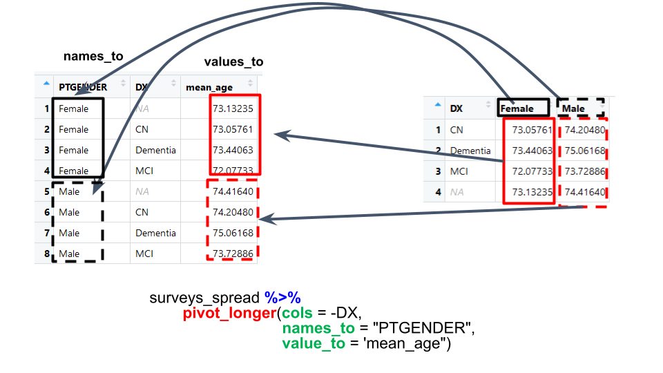
Creating long data
The opposing situation could occur if we had been provided with data in the
form of adni_r_DXS_wide, where the diagnoses are column names, but we
wish to treat them as values of a diagnosis variable instead.
In this situation we are turning the column names into a pair of new variables. One variable represents the column names as values, and the other variable contains the values previously associated with the column names.
pivot_longer() takes four principal arguments:
- the data
- cols : Columns to pivot into longer format.
- names_to: column to create from column names.
- values_to: column to fill with values
- the names of the columns we use to fill the key variable (or to drop).
To recreate adni_r_DXS from adni_r_DXS_wide we would create a key called
PTGENDER and value called mean_age and use all columns except DX for
the key variable. Here we drop DX column with a minus sign.
adni_r_long <- adni_r_DXS_wide %>%
  pivot_longer(cols = -DX , names_to = "PTGENDER", values_to = "mean_age" )

adni_r_long
# A tibble: 8 x 3
  DX       PTGENDER mean_age
  <chr>    <chr>       <dbl>
1 CN       Female       73.1
2 CN       Male         74.2
3 Dementia Female       73.4
4 Dementia Male         75.1
5 MCI      Female       72.1
6 MCI      Male         73.7
7 <NA>     Female       73.1
8 <NA>     Male         74.4
A different way to write the cols parameter is to specify what to include (the male and female columns) instead of specifying what to exclude (the DX column). This strategy can be
useful if you have a large number of columns but you only want to include a few of them in the new table. If the columns are in a row, we don’t even need to list them all out - just use the : operator!
adni_r_long <- adni_r_DXS_wide %>%
  pivot_longer(cols = Male:Female , names_to = "PTGENDER", values_to = "mean_age" )

adni_r_long
# A tibble: 8 x 3
  DX       PTGENDER mean_age
  <chr>    <chr>       <dbl>
1 CN       Male         74.2
2 CN       Female       73.1
3 Dementia Male         75.1
4 Dementia Female       73.4
5 MCI      Male         73.7
6 MCI      Female       72.1
7 <NA>     Male         74.4
8 <NA>     Female       73.1
Challenge
- Create a data frame (from the
adni_rdataset using summarize) with the number of patients of each gender seen at each site. You will need to use the functionn_distinct()to get the number of unique patients within a particular chunk of data. It’s a powerful function! See ?n_distinct for more. Then pivot that data frame to the wide form where genders are the columns.Solution
site_gender <- adni_r %>%
  group_by(SITE, PTGENDER) %>%
  summarize(n_pt = n_distinct(PTID)) %>%
  pivot_wider(names_from = PTGENDER,
              values_from = n_pt)

head(site_gender)
# A tibble: 6 x 3 # Groups: SITE [6] SITE Female Male <dbl> <int> <int> 1 2 28 21 2 3 26 21 3 5 9 15 4 6 12 25 5 7 21 19 6 9 11 21
- The
adni_rdata set has many measurement columns, for exampleAGE_modandPTEDUCAT. This makes it difficult to do things like look at the relationship between mean values of each measurement per year in different plot types. Let’s walk through a common solution for this type of problem. First, usepivot_longer()to create a dataset where we have a key column calledmeasurementand avaluecolumn that takes on the value of eitherAGE_modorPTEDUCAT.Solution
adni_r_long <- adni_r %>%
  pivot_longer(names_to = "measurement",
               values_to = "value",
               c(AGE_mod, PTEDUCAT)) #columns to reshape
- With this new data set, calculate the average of each
measurementin eachyearfor each differentSITE. Then usepivot_wider()to create a data set with a column for each measurement.Solution
adni_r_long %>%
  group_by(year, measurement, SITE) %>%
  summarize(mean_value = mean(value, na.rm=TRUE)) %>%
  pivot_wider(names_from = measurement,
              values_from = mean_value)
# A tibble: 788 x 4 # Groups: year [15] year SITE AGE_mod PTEDUCAT <dbl> <dbl> <dbl> <dbl> 1 2005 7 73.0 14.7 2 2005 11 74.1 15 3 2005 18 76.4 20 4 2005 22 76.3 13.2 5 2005 23 76.9 17.5 6 2005 35 83.3 20 7 2005 67 70.9 14.8 8 2005 99 73.6 18.7 9 2005 100 79.4 16.3 10 2005 123 74.2 15 # … with 778 more rows
Exporting data
Now that you have learned how to use dplyr to extract information from
or summarize your raw data, you may want to export these new data sets to share
them with your collaborators or for archival.
Similar to the read_csv() function used for reading CSV files into R, there is
a write_csv() function that generates CSV files from data frames.
Before using write_csv(), we are going to create a new folder, data_output,
in our working directory that will store this generated dataset. We don’t want
to write generated datasets in the same directory as our raw data. It’s good
practice to keep them separate. The data folder should only contain the raw,
unaltered data, and should be left alone to make sure we don’t delete or modify
it. In contrast, our script will generate the contents of the data_output
directory, so even if the files it contains are deleted, we can always
re-generate them.
Because we have added date columns to the dataset, we can save it as a CSV file in our data_output folder using write_csv.
write_csv(adni_r, path = "data_output/adni_r_dates.csv")
Key Points