Reproducible Reports with RMarkdown
Overview
Teaching: min
Exercises: minQuestions
How can I make reproducible reports in R?
Objectives
Describe how RMarkdown can be used to generate reproducible reports.
Apply Markdown features such as bulleting, italics, bold font, numbered lists.
Use code chunks and code chunk options within an RMarkdown document.
Set inline R code.
Build a reproducible document that outputs to an HTML file.
Material adapted from Reproducible Reports with R Markdown - Karl Broman and R programming: R Reports - Tobin Magle.
Why RMarkdown?
RMarkdown is a type of literate programming, which lets you combine human-readable text and machine-readable code to produce a reproducible document. Literate programming is the idea that instead of writing code to tell the computer what to do, you should write code as if you are telling another human what you want the computer to do. This strategy can improve the documentation of your code and the usability of the code itself.
Literate program lets you do many things that are useful in research:
- combine text, code, figures, tables all in one reproducible document
- tailor reports to different audiences
- use version control and with programming languages commonly used in research like R and python
Today we’re going to look at RMarkdown to do literate programming in R Studio, though it does work with other programming languages like python and stata. It can also produce outputs in many formats like Microsoft Word documents, PDFs, slides, and HTML files for the web.
You can create output in many document formats without having to remember to swap figures, change cell values in tables, or values in text using RMarkdown, all by changing a single line of code! In fact, this lesson material is written in RMarkdown!
Scenario
You work in a research group that has been collecting the ADNI dataset. You do all your analysis in R.Your funder wants a yearly report summarizing the data in .docx format.
Goal: Write an R Markdown report that you can run yearly on the data for your funder. They want the following information in the report:
- A paragraph summarizing the data: total # of patients, total # of diagnoses represented in the surveys, and what variables were measured:
This dataset has a total of 1656 patients and measures 8 variables: PTID, AGE, PTGENDER, DX, WholeBrain, Hippocampus, APOE4, exam_year. These observations included the following diagnoses: CN, Dementia, MCI, NA.
- A table of the number of observations by
PTGENDERandDX:
| PTGENDER | DX | n |
|---|---|---|
| Female | CN | 933 |
| Female | Dementia | 565 |
| Female | MCI | 1121 |
| Female | NA | 314 |
| Male | CN | 972 |
| Male | Dementia | 718 |
| Male | MCI | 1657 |
| Male | NA | 357 |
- A scatter plot of Whole brain volume vs. hippocampus volume, colored by
PTGENDER:

Creating an RMarkdown Document
To create a new RMarkdown document, in RStudio, navigate to File, then New File, and finally click on R Markdown.
RStudio -> File -> New File ->R Markdown (keep defaults, add title)
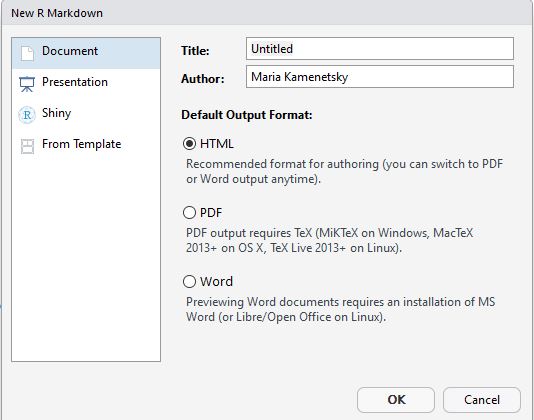
Keep the defaults for now and add your own title. In this lesson, we will keep the default output format as HTML. However if you have LaTeX installed, you can also create PDF documents.
Parts of an R Markdown document
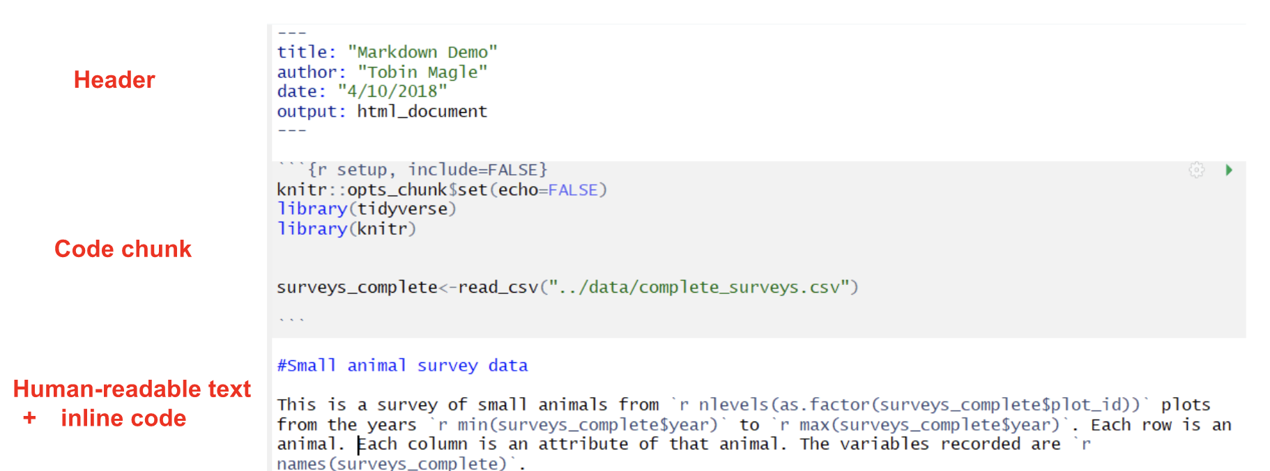
R Markdown documents are made of 3 basic parts:
- The header lets you set options for the document. Notice here that the title you gave the document appears here along with your name, the current date, and the output format (HTML).
- Human readable text lets you write the narrative of the report in the Markdown language
- Code chunks allow you to embed R code and/or output into your document. We’ll cover how to decide what to include in the document later.
- Inline code allows you to calculate values based on the data within the human readable text
Rendering an RMarkdown Document
To render your RMarkdown document to html, click small yarn and knitting needle icon labeled ‘Knit’. If you click the black arrow to the right, you can also see some of the other options for output formats that you can knit to, such as PDF and Word. Note that you may need to install additional software on your computer (Microsoft Word for Word, and LaTeX for PDFs)
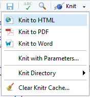
After knitting the document, (if it was successful) a preview of the html document will show up in the preview pane of RStudio.

How this works
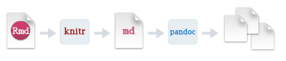
There are several tools that work together to produce your final document.
The
RMarkdownfile will be sent toknitr. In turn,knitrwill knit together your
text and code and send that toMarkdownto for text formatting. Then,pandocwill convert the markdown document with text and code to create the final output format.
Markdown Syntax
The following is a table of the basic Markdown syntax along with how the rendered output looks. A cheatsheet of Markdown syntax provided by RStudio can be found on their website.
| Description |
Markdown Syntax |
Rendered Output |
|---|---|---|
| Headers |
# Header 1 ## Header 2 ### Header 3 |
Header 1 Header 2 Header 3 |
| Bolded Statements |
**a bolded statement** |
a bolded statement |
| Italicized Statement |
*an italicized statement* | an italicized statement |
| Code Font |
`code-type font` |
code-type font |
You can also make lists with the following
Bulleted List
* item
* item

Numbered List
1. ordered item
2. ordered item
So if we include the following Markdown code in our document
## Reflections on Markdown So Far

Markdown is **super** awesome, I'm *not* even joking.

Why I love `RMarkdown`:

1. It makes things reproducible
2. Easy to collaborate
3. It's fun!
We will get output that looks like this
Reflections on Markdown So Far
Markdown is super awesome, I’m not even joking.
Why I love
RMarkdown:
- It makes things reproducible
- Easy to collaborate
- It’s fun!
Advanced Markdown Features
More advanced formatting can be used in Markdown, such as including links, images, and even LaTeX formulas:
| Add a hyperlink | [text to show](http://the-web-page.com) | text to show |
| Include an image |  |  |
| Subscript and Super Script | F~2~` and `F^2 | \(F_2\) and \(F^2\) |
| LaTeX Inline Math | `$E=mc^2$` | \(E=mc^2\) |
| LaTeX Display Math |
$$y = \mu + \sum_{i=1}^p \beta_i x_i + \epsilon$$ | $$y = \mu + \sum_{i=1}^p \beta_i x_i + \epsilon$$ |
Challenge 1
Literate programming in action
Let’s start by writing a human readable outline of our document.
Make a new RMarkdown document if you haven’t already. Delete all of the R code chunks and text (except the header). Create an outline for your report. Example below:
Summary
This dataset has a total of ## patients and measures ## variables:
. These observations included the following diagnoses: . Count table by
PTGENDERandDXinsert table here
Whole brain volume vs. hippocampus volume, colored by
PTGENDERinsert plot here
Knit to HTML.
R code chunks
An R code chunk begins with three backticks followed by a lower case r in brackets. The code chunk ends with three backticks. The code goes in the middle.
```{r}
R code goes here
```
In RMarkdown, you will notice the code chunk because it will appear grey in your document.
Shortcut
You can create a new code chunk manually (with backticks) or use the short-cut: CTRL+ALT+i.
Let’s use a code chunk to load the ADNI data and tidyverse packages into our RMarkdown document.
```{r}
library(tidyverse)
adni_c <- read_csv("data/processed_data/adni_clean.csv")
```
You should also give each code chunk a name, which can help you organize the contents of your Rmarkdown document and find errors when the document is rendered:
```{r setup-chunk}
library(tidyverse)
adni_c <- read_csv("data/adni_clean.csv")
```
Challenge
Add code chunks to display the plot requested by the funders in your outline.
Solution
# Whole brain volume vs. hippocampus volume, colored by `PTGENDER````{r rmd-plot} ggplot(data = adni_c, mapping = aes(x = Hippocampus, y = WholeBrain)) + geom_point(alpha = 0.5, aes(color = PTGENDER)) ```
Code chunk options
You may have noticed that when you knit your document, you see the code, plot, and warning messages. We can use code chunk options to control what is displayed in the document.
There are many different code chunk options and a full list can be found here. Some of the most frequently used chunk options are:
- `echo=FALSE`: suppress code from being printed in final report
- `include = FALSE`: prevents code and results from appearing in the finished file. R Markdown still runs the code in the chunk, and the results can be used by other chunks.
- `eval=FALSE`: do not evaluate the code chunk.
- `warning=FALSE` and `message=FALSE` hides any warnings or messages produced.
- `fig.height`, `fig.width` controls size of figures (in inches).
- `fig.cap`: adds a caption to the figures.
Code chunk options can be set locally (for each code chunk individually) or globally (for the entire RMarkdown document)
Using code chunk options in a code chunk
We can control local code chunks with code chunk options. Let’s edit the setup code chunk so that it doesn’t display code or output from loading the file and packages:
```{r setup, include = FALSE}
library(tidyverse)
adni_c <- read_csv("data/processed_data/adni_clean.csv")
```
Setting code chunk options globally
If you want the output for all of your code chunks to be the same, you can set these preferences globally. A global code chunk will look like this if you wanted the code, warnings and messages to be excluded, but the output to be displayed.
```{r setupexample, include=FALSE}
knitr::opts_chunk$set(echo=FALSE, warning = FALSE, message = FALSE)
```
Settings in the code chunks will override these global settings
Challenge
Use chunk options to control to hide the code for the plot code chunk.
Solution
```{r rmd-plot, echo = FALSE}
ggplot(data = adni_c,
      mapping = aes(x = Hippocampus,
                    y = WholeBrain)) +
   geom_point(alpha = 0.5,
              aes(color = PTGENDER))
```
Inline R Code
In RMarkdown, you can also also include some R code as inside your text, making every number in your report reproducible in the text. The syntax for
inline code looks like this:
`r code_goes_here `
For example:
Pi rounded to 2 decimal places is `r round(3.14159, 2)`
Would Evaluate to
Pi rounded to 2 decimal places is 3.14
Complex calculations inline
If you have some calculations to do, you can have a preceding R chunk to calculate the results and store it in a variable. Hide the code and results using
include=FALSE. Then you can print the variable in the inline code.
Challenge
Place inline code in the summary paragraph to calculate the values that currently have placeholders.
Solution
This dataset has a total of 1656 patients and measures 8 variables: PTID, AGE, PTGENDER, DX, WholeBrain, Hippocampus, APOE4, exam_year. These observations included the following diagnoses: CN, Dementia, MCI, NA.
Tables
R will display data frames and matrices in your report as it would in the console:
adni_c%>%
  distinct(PTID, PTGENDER, DX)%>%
  count(PTGENDER, DX)
# A tibble: 8 x 3
  PTGENDER DX           n
  <chr>    <chr>    <int>
1 Female   CN         278
2 Female   Dementia   237
3 Female   MCI        362
4 Female   <NA>       313
5 Male     CN         273
6 Male     Dementia   310
7 Male     MCI        518
8 Male     <NA>       353
For more flexibility in formatting tables, you can the kable() function from the knitr package.
library(knitr)
kable(adni_c%>%
  distinct(PTID, PTGENDER, DX)%>%
  count(PTGENDER, DX))
| PTGENDER | DX | n |
|---|---|---|
| Female | CN | 278 |
| Female | Dementia | 237 |
| Female | MCI | 362 |
| Female | NA | 313 |
| Male | CN | 273 |
| Male | Dementia | 310 |
| Male | MCI | 518 |
| Male | NA | 353 |
Challenge
Use the
kablefunction to add the table to the document and set the code chunk options so that the code doesn’tSolution
kable(adni_c%>%
 distinct(PTID, PTGENDER, DX)%>%
 count(PTGENDER, DX))
PTGENDER DX n Female CN 278 Female Dementia 237 Female MCI 362 Female NA 313 Male CN 273 Male Dementia 310 Male MCI 518 Male NA 353
Resources
We’ve just touched the surface of how useful Rmarkdown can be in creating reproducible reports. Please see some of these other resources for more details!
- Knitr in a knutshell tutorial
- Dynamic Documents with R and knitr (book)
- R Markdown documentation
- R Markdown cheat sheet
- Creating Awesome Tables with kable and kableExtra
Key Points