Intro to Raster Data in R
Overview
Teaching: 40 min
Exercises: 20 minQuestions
What is a raster dataset?
How do I work with and plot raster data in R?
How can I handle missing or bad data values for a raster?
Objectives
Describe the fundamental attributes of a raster dataset.
Explore raster attributes and metadata using R.
Import rasters into R using the
rasterpackage.Plot a raster file in R using the
ggplot2package.Describe the difference between single- and multi-band rasters.
In this episode, we will introduce the fundamental principles, packages and metadata/raster attributes that are needed to work with raster data in R. We will discuss some of the core metadata elements that we need to understand to work with rasters in R, including CRS and resolution. We will also explore missing and bad data values as stored in a raster and how R handles these elements.
We will continue to work with the dplyr and ggplot2 packages that were introduced
in the Introduction to R for Geospatial Data lesson. We will use two additional packages in this episode to work with raster data - the
raster and rgdal packages. Make sure that you have these packages loaded.
library(raster)
library(rgdal)
##The Data
In this lesson, we will be working with two field sites: the Harvard Forest (HARV) and San Joaquin Experimental Range (SJER).
In this lesson, the raster we will use is: HARV_dsmCrop.tif.
For the challenges in this lesson, we will use both and HARV_dsmCrop.tif and HARV_DSMhill.tif.
View Raster File Attributes
We will be working with a series of GeoTIFF files in this lesson. The
GeoTIFF format contains a set of embedded tags with metadata about the raster
data. We can use the function GDALinfo() to get information about our raster
data before we read that data into R. It is ideal to do this before importing
your data.
GDALinfo("data/raster/HARV_dsmCrop.tif")
rows        898
columns     1078
bands       1
lower left origin.x        731453
lower left origin.y        4712472
res.x       1
res.y       1
ysign       -1
oblique.x   0
oblique.y   0
driver      GTiff
projection  +proj=utm +zone=18 +datum=WGS84 +units=m +no_defs
file        data/raster/HARV_dsmCrop.tif
apparent band summary:
   GDType hasNoDataValue NoDataValue blockSize1 blockSize2
1 Float32           TRUE    -3.4e+38          1       1078
apparent band statistics:
   Bmin   Bmax    Bmean      Bsd
1 330.9 405.15 370.6424 14.27794
Metadata:
AREA_OR_POINT=Area
If you wish to store this information in R, you can do the following:
HARV_dsmCrop_info <- capture.output(
  GDALinfo("data/raster/HARV_dsmCrop.tif")
)
HARV_dsmCrop_info
 [1] "rows        898 "
 [2] "columns     1078 "
 [3] "bands       1 "
 [4] "lower left origin.x        731453 "
 [5] "lower left origin.y        4712472 "
 [6] "res.x       1 "
 [7] "res.y       1 "
 [8] "ysign       -1 "
 [9] "oblique.x   0 "
[10] "oblique.y   0 "
[11] "driver      GTiff "
[12] "projection  +proj=utm +zone=18 +datum=WGS84 +units=m +no_defs "
[13] "file        data/raster/HARV_dsmCrop.tif "
[14] "apparent band summary:"
[15] "   GDType hasNoDataValue NoDataValue blockSize1 blockSize2"
[16] "1 Float32           TRUE    -3.4e+38          1       1078"
[17] "apparent band statistics:"
[18] "   Bmin   Bmax    Bmean      Bsd"
[19] "1 330.9 405.15 370.6424 14.27794"
[20] "Metadata:"
[21] "AREA_OR_POINT=Area "
Each line of text that was printed to the console is now stored as an element of
the character vector HARV_dsmCrop_info. We will be exploring this data throughout this
episode. By the end of this episode, you will be able to explain and understand the output above.
Open a Raster in R
Now that we’ve previewed the metadata for our GeoTIFF, let’s import this
raster dataset into R and explore its metadata more closely. We can use the raster()
function to open a raster in R.
First we will load our raster file into R and view the data structure.
DSM_HARV <- raster("data/raster/HARV_dsmCrop.tif")

DSM_HARV
class      : RasterLayer
dimensions : 898, 1078, 968044  (nrow, ncol, ncell)
resolution : 1, 1  (x, y)
extent     : 731453, 732531, 4712472, 4713370  (xmin, xmax, ymin, ymax)
crs        : +proj=utm +zone=18 +datum=WGS84 +units=m +no_defs +ellps=WGS84 +towgs84=0,0,0
source     : /home/travis/build/UW-Madison-DataScience/r-raster-vector-geospatial/_episodes_rmd/data/raster/HARV_dsmCrop.tif
names      : HARV_dsmCrop
values     : 330.9, 405.15  (min, max)
The information above includes a report of min and max values, but no other data range statistics. Similar to other R data structures like vectors and data frame columns, descriptive statistics for raster data can be retrieved like
summary(DSM_HARV)
Warning in .local(object, ...): summary is an estimate based on a sample of 1e+05 cells (10.33% of all cells)
        HARV_dsmCrop
Min.          331.05
1st Qu.       361.58
Median        372.57
3rd Qu.       380.80
Max.          404.77
NA's            0.00
but note the warning - unless you force R to calculate these statistics using
every cell in the raster, it will take a random sample of 100,000 cells and
calculate from that instead. To force calculation on more, or even all values,
you can use the parameter maxsamp:
summary(DSM_HARV, maxsamp = ncell(DSM_HARV))
        HARV_dsmCrop
Min.          330.90
1st Qu.       361.52
Median        372.52
3rd Qu.       380.84
Max.          405.15
NA's            0.00
You may not see major differences in summary stats as maxsamp increases,
except with very large rasters.
To visualise this data in R using ggplot2, we need to convert it to a
dataframe.
The raster package has an built-in function for conversion to a plotable dataframe.
DSM_HARV_df <- as.data.frame(DSM_HARV, xy = TRUE)
Now when we view the structure of our data, we will see a standard
dataframe format. We can apply str to view the structure of the new dataframe, DSM_HARV_df
str(DSM_HARV_df)
'data.frame':	968044 obs. of  3 variables:
 $ x           : num  731454 731454 731456 731456 731458 ...
 $ y           : num  4713370 4713370 4713370 4713370 4713370 ...
 $ HARV_dsmCrop: num  370 371 371 362 370 ...
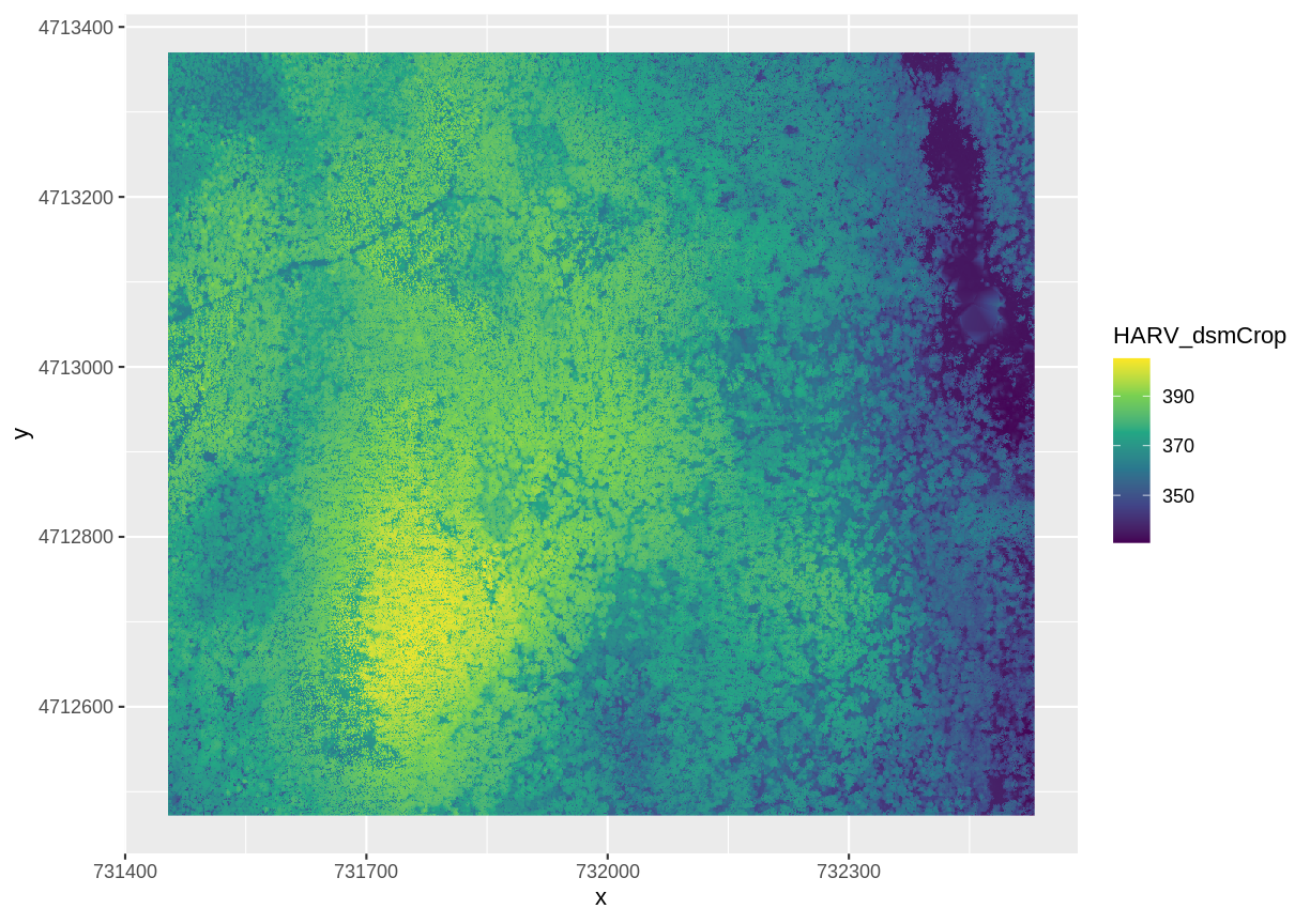
We can use ggplot() to plot this data. We will set the color scale to scale_fill_viridis_c
which is a color-blindness friendly color scale. We will also use the coord_quickmap() function to use an approximate Mercator projection for our plots. This approximation is suitable for small areas that are not too close to the poles. Other coordinate systems are available in ggplot2 if needed, you can learn about them at their help page ?coord_map.
ggplot() +
    geom_raster(data = DSM_HARV_df , aes(x = x, y = y, fill = HARV_dsmCrop)) +
    scale_fill_viridis_c() +
    coord_quickmap()

This map shows the elevation of our study site in Harvard Forest. From the legend, we can see that the maximum elevation is ~400, but we can’t tell whether this is 400 feet or 400 meters because the legend doesn’t show us the units. We can look at the metadata of our object to see what the units are. Much of the metadata that we’re interested in is part of the CRS..
Now we will see how features of the CRS appear in our data file and what meanings they have.
View Raster Coordinate Reference System (CRS) in R
We can view the CRS string associated with our R object using thecrs()
function.
crs(DSM_HARV)
CRS arguments:
 +proj=utm +zone=18 +datum=WGS84 +units=m +no_defs +ellps=WGS84
+towgs84=0,0,0
Challenge
What units are our data in?
Answers
+units=mtells us that our data is in meters.
Understanding CRS in Proj4 Format
The CRS for our data is given to us by R in proj4 format. Let’s break down
the pieces of proj4 string. The string contains all of the individual CRS
elements that R or another GIS might need. Each element is specified with a
+ sign, similar to how a .csv file is delimited or broken up by a ,. After
each + we see the CRS element being defined. For example projection (proj=)
and datum (datum=).
UTM Proj4 String
Our projection string for DSM_HARV specifies the UTM projection as follows:
+proj=utm +zone=18 +datum=WGS84 +units=m +no_defs +ellps=WGS84 +towgs84=0,0,0
- proj=utm: the projection is UTM, UTM has several zones.
- zone=18: the zone is 18
- datum=WGS84: the datum is WGS84 (the datum refers to the 0,0 reference for the coordinate system used in the projection)
- units=m: the units for the coordinates are in meters
- ellps=WGS84: the ellipsoid (how the earth’s roundness is calculated) for the data is WGS84
Note that the zone is unique to the UTM projection. Not all CRS’s will have a zone. Image source: Chrismurf at English Wikipedia, via Wikimedia Commons (CC-BY).
Calculate Raster Min and Max Values
It is useful to know the minimum or maximum values of a raster dataset. In this case, given we are working with elevation data, these values represent the min/max elevation range at our site.
Raster statistics are often calculated and embedded in a GeoTIFF for us. We can view these values:
minValue(DSM_HARV)
[1] 330.9
maxValue(DSM_HARV)
[1] 405.15
Since the minimum and maximum values haven’t already been calculated, we can calculate them using the setMinMax() function.
DSM_HARV <- setMinMax(DSM_HARV)
minValue(DSM_HARV)
[1] 330.9
maxValue(DSM_HARV)
[1] 405.15
Raster Bands
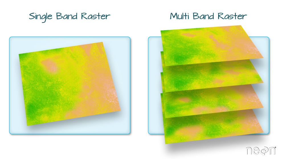
The Digital Surface Model object (DSM_HARV) that we’ve been working with is a
single band raster. This means that there is only one dataset stored in the
raster: surface elevation in meters for one time period.

A raster dataset can contain one or more bands. We can use the raster()
function to import one single band from a single or multi-band raster. We can
view the number of bands in a raster using the nlayers() function.
nlayers(DSM_HARV)
[1] 1
However, raster data can also be multi-band, meaning that one raster file
contains data for more than one variable or time period for each cell. By
default the raster() function only imports the first band in a raster
regardless of whether it has one or more bands.
##Missing Data
The value that is conventionally used to take note of missing data (the
NoDataValue value) varies by the raster data type. For floating-point rasters,
the figure -3.4e+38 is a common default, and for integers, -9999 is
common. Some disciplines have specific conventions that vary from these
common values.
In some cases, other NA values may be more appropriate. An NA value should
be a) outside the range of valid values, and b) a value that fits the data type
in use. For instance, if your data ranges continuously from -20 to 100, 0 is
not an acceptable NA value! Or, for categories that number 1-15, 0 might be
fine for NA, but using -.000003 will force you to save the GeoTIFF on disk
as a floating point raster, resulting in a bigger file.
If we are lucky, our GeoTIFF file has a tag that tells us what is the
NoDataValue. If we are less lucky, we can find that information in the
raster’s metadata. If a NoDataValue was stored in the GeoTIFF tag, when R
opens up the raster, it will assign each instance of the value to NA. Values
of NA will be ignored by R as demonstrated above.
Challenge
Use the output from the
GDALinfo()function to find out whatNoDataValueis used for ourDSM_HARVdataset.Answers
GDALinfo("data/raster/HARV_dsmCrop.tif")rows 898 columns 1078 bands 1 lower left origin.x 731453 lower left origin.y 4712472 res.x 1 res.y 1 ysign -1 oblique.x 0 oblique.y 0 driver GTiff projection +proj=utm +zone=18 +datum=WGS84 +units=m +no_defs file data/raster/HARV_dsmCrop.tif apparent band summary: GDType hasNoDataValue NoDataValue blockSize1 blockSize2 1 Float32 TRUE -3.4e+38 1 1078 apparent band statistics: Bmin Bmax Bmean Bsd 1 330.9 405.15 370.6424 14.27794 Metadata: AREA_OR_POINT=Area
NoDataValueare encoded as -9999.
Create A Histogram of Raster Values
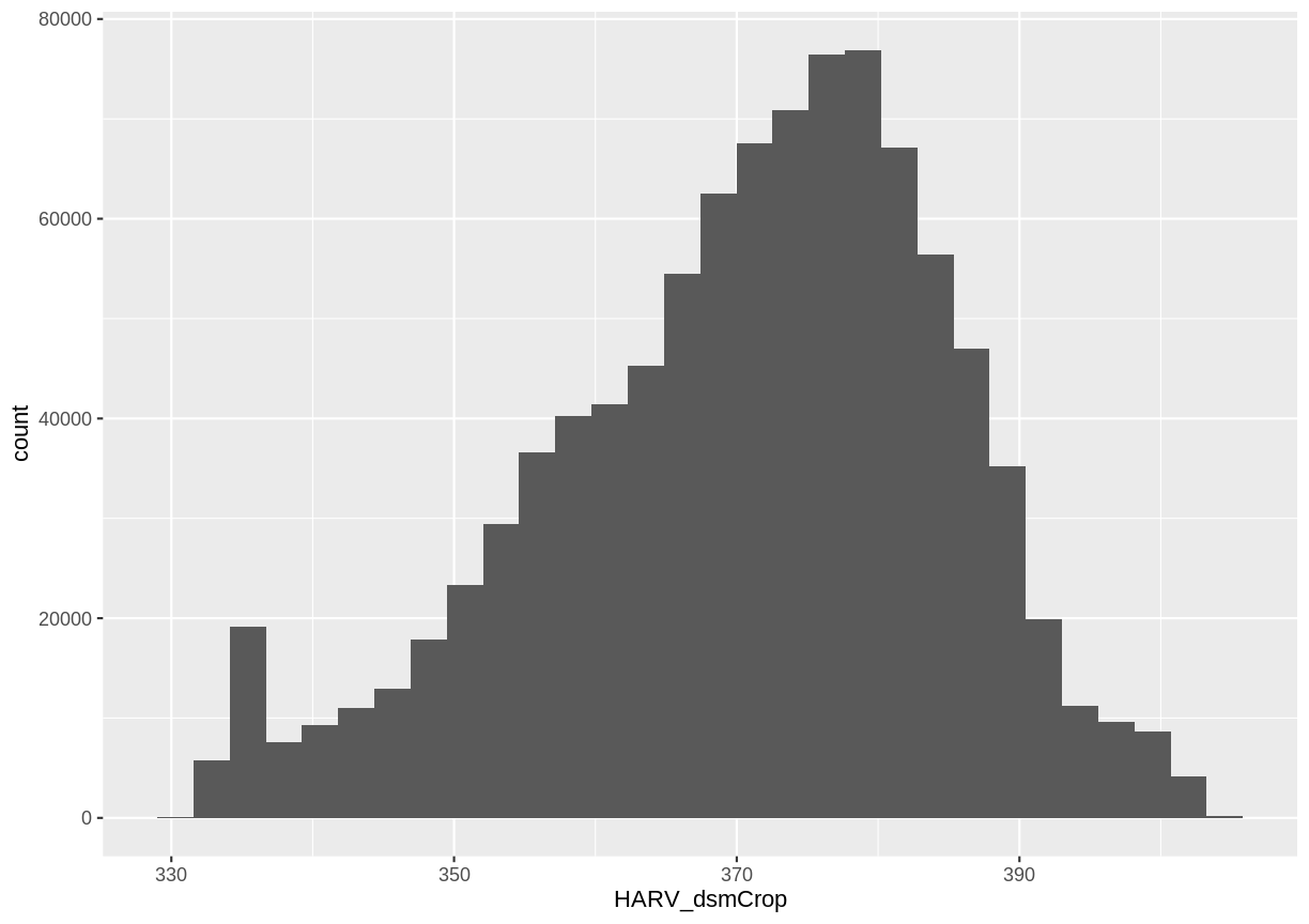
We can explore the distribution of values contained within our raster using the
geom_histogram() function which produces a histogram. Histograms are often
useful in identifying outliers and bad data values in our raster data.
ggplot() +
    geom_histogram(data = DSM_HARV_df, aes(HARV_dsmCrop))
`stat_bin()` using `bins = 30`. Pick better value with `binwidth`.

Notice that a warning message is thrown when R creates the histogram.
stat_bin() using bins = 30. We could pick a better bin value with the argument binwidth.
Challenge: Explore Raster Metadata
Use
GDALinfo()to determine the following about thedata/raster/HARV_DSMhill.tiffile:
- Does this file have the same CRS as
DSM_HARV?- What is the
NoDataValue?- What is resolution of the raster data?
- How large would a 5x5 pixel area be on the Earth’s surface?
- Is the file a multi- or single-band raster?
Notice: this file is a hillshade. We will learn about hillshades in the Working with Multi-band Rasters in R episode.
Answers
GDALinfo("data/raster/HARV_DSMhill.tif")rows 898 columns 1078 bands 1 lower left origin.x 731453 lower left origin.y 4712472 res.x 1 res.y 1 ysign -1 oblique.x 0 oblique.y 0 driver GTiff projection +proj=utm +zone=18 +datum=WGS84 +units=m +no_defs file data/raster/HARV_DSMhill.tif apparent band summary: GDType hasNoDataValue NoDataValue blockSize1 blockSize2 1 Float32 TRUE -3.4e+38 1 1078 apparent band statistics: Bmin Bmax Bmean Bsd 1 -0.7131745 0.9999997 0.2932656 0.487991 Metadata: AREA_OR_POINT=Area
- If this file has the same CRS as DSM_HARV? Yes: UTM Zone 18, WGS84, meters.
- What format
NoDataValuestake? -3.4e+38- The resolution of the raster data? 1x1
- How large a 5x5 pixel area would be? 5mx5m How? We are given resolution of 1x1 and units in meters, therefore resolution of 5x5 means 5x5m.
- Is the file a multi- or single-band raster? Single.
More Resources
Key Points
The GeoTIFF file format includes metadata about the raster data.
To plot raster data with the
ggplot2package, we need to convert it to a dataframe.R stores CRS information in the Proj4 format.
Be careful when dealing with missing or bad data values.
