Manipulate Raster Data in R
Overview
Teaching: 40 min
Exercises: 20 minQuestions
How can I crop raster objects to vector objects, and extract the summary of raster pixels?
Objectives
Crop a raster to the extent of a vector layer.
Extract values from a raster that correspond to a vector file overlay.
Things You’ll Need To Complete This Episode
See the lesson homepage for detailed information about the software, data, and other prerequisites you will need to work through the examples in this episode.
This episode explains how to crop a raster using the extent of a vector shapefile. We will also cover how to extract values from a raster that occur within a set of polygons, or in a buffer (surrounding) region around a set of points.
We will continue to work with specific packages for working with spatial data. Let’s load all of the packages we have been working with in this lesson.
library(sf)
library(raster)
library(rgdal)
library(ggplot2)
library(dplyr)
We will also continue to work with the HARV vector data. You may have these layers already loaded into your enviroment, but if not, load them now.
Crop a Raster to Vector Extent
We often work with spatial layers that have different spatial extents. The spatial extent of a shapefile or R spatial object represents the geographic “edge” or location that is the furthest north, south east and west. Thus is represents the overall geographic coverage of the spatial object.
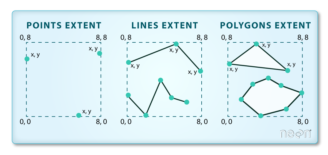 Image Source: National
Ecological Observatory Network (NEON)
Image Source: National
Ecological Observatory Network (NEON)
The graphic below illustrates the extent of several of the spatial layers that we have worked with in this workshop:
- Area of interest (AOI) – blue
- Roads and trails – purple
- Vegetation plot locations (marked with white dots)– black
- A canopy height model (CHM) in GeoTIFF format – green

Frequent use cases of cropping a raster file include reducing file size and creating maps. Sometimes we have a raster file that is much larger than our study area or area of interest. It is often more efficient to crop the raster to the extent of our study area to reduce file sizes as we process our data. Cropping a raster can also be useful when creating pretty maps so that the raster layer matches the extent of the desired vector layers.
Crop a Raster Using Vector Extent
We can use the crop() function to crop a raster to the extent of another
spatial object. To do this, we need to specify the raster to be cropped and the
spatial object that will be used to crop the raster. R will use the extent of
the spatial object as the cropping boundary.
To illustrate this, we will crop the Canopy Height Model (CHM) to only include the area of interest (AOI). Let’s start by plotting the full extent of the CHM data and overlay where the AOI falls within it. The boundaries of the AOI will be colored blue, and we use fill = NA to make the area transparent.
ggplot() +
  geom_raster(data = CHM_HARV_df, aes(x = x, y = y, fill = HARV_chmCrop)) +
  geom_sf(data = aoi_boundary_HARV, color = "blue", fill = NA) +
  coord_sf()

Now that we have visualized the area of the CHM we want to subset, we can
perform the cropping operation. We are going to crop() function from the
raster package to create a new object with only the portion of the CHM data
that falls within the boundaries of the AOI.
CHM_HARV_Cropped <- crop(x = CHM_HARV, y = aoi_boundary_HARV)
Now we can plot the cropped CHM data, along with a boundary box showing the full
CHM extent. However, remember, since this is raster data, we need to convert to
a data frame in order to plot using ggplot.
For this plot, I am going to do a little trick to add the extent of the CHM to our plot, without creating a spatial extent object and without including the actual CHM in the plot. To get the spatial extent, I am going to use the st_bbox() function. This stands for bounding box, and the function will extract the 4 corners of the rectangle that encompass all the features contained in this object. I will also use the function st_as_sfc that we saw before to convert the extent into a spatial object that we can include in our plot. All of this will happen within the geom_sf function in our ggplot code.
CHM_HARV_Cropped_df <- as.data.frame(CHM_HARV_Cropped, xy = TRUE)

ggplot() +
  geom_sf(data = st_as_sfc(st_bbox(CHM_HARV)), fill = "green",
          color = "green", alpha = .2) +
  geom_raster(data = CHM_HARV_Cropped_df,
              aes(x = x, y = y, fill = HARV_chmCrop)) +
  coord_sf()

The plot above shows that the full CHM extent (plotted in green) is much larger
than the resulting cropped raster. Our new cropped CHM now has the same extent
as the aoi_boundary_HARV object that was used as a crop extent (blue border
below).
ggplot() +
  geom_raster(data = CHM_HARV_Cropped_df,
              aes(x = x, y = y, fill = HARV_chmCrop)) +
  geom_sf(data = aoi_boundary_HARV, color = "blue", fill = NA) +
  scale_fill_gradientn(name = "Canopy Height", colors = terrain.colors(10)) +
  coord_sf()

Challenge: Crop to Vector Points Extent
- Crop the Canopy Height Model to the extent of the study plot locations.
- Plot the vegetation plot location points on top of the Canopy Height Model.
Answers
CHM_plots_HARVcrop <- crop(x = CHM_HARV, y = plot_locations_sp_HARV)

CHM_plots_HARVcrop_df <- as.data.frame(CHM_plots_HARVcrop, xy = TRUE)

ggplot() +
  geom_raster(data = CHM_plots_HARVcrop_df, aes(x = x, y = y, fill = HARV_chmCrop)) +
  scale_fill_gradientn(name = "Canopy Height", colors = terrain.colors(10)) +
  geom_sf(data = plot_locations_sp_HARV) +
  coord_sf()

In the plot above, created in the challenge, all the vegetation plot locations (black dots) appear on the Canopy Height Model raster layer except for one. One is situated on the blank space to the left of the map. Why?
A modification of the first figure in this episode is below, showing the
relative extents of all the spatial objects. Notice that the extent for our
vegetation plot layer (black) extends further west than the extent of our CHM
raster (bright green). The crop() function will make a raster extent smaller, it
will not expand the extent in areas where there are no data. Thus, the extent of our
vegetation plot layer will still extend further west than the extent of our
(cropped) raster data (dark green).
Define an Extent
So far, we have used a shapefile to crop the extent of a raster dataset.
Alternatively, we can also the extent() function to define an extent to be
used as a cropping boundary. This creates a new object of class extent. Here we
will provide the extent() function our xmin, xmax, ymin, and ymax (in that
order).
new_extent <- extent(732161.2, 732238.7, 4713249, 4713333)
class(new_extent)
[1] "Extent"
attr(,"package")
[1] "raster"
Data Tip
The extent can be created from a numeric vector (as shown above), a matrix, or a list. For more details see the
extent()function help file (?raster::extent).
Once we have defined our new extent, we can use the crop() function to crop
our raster to this extent object.
CHM_HARV_manual_cropped <- crop(x = CHM_HARV, y = new_extent)
To plot this data using ggplot() we need to convert it to a dataframe.
CHM_HARV_manual_cropped_df <- as.data.frame(CHM_HARV_manual_cropped, xy = TRUE)
Now we can plot this cropped data. We will show the AOI boundary on the same plot for scale.
ggplot() +
  geom_sf(data = aoi_boundary_HARV, color = "blue", fill = NA) +
  geom_raster(data = CHM_HARV_manual_cropped_df,
              aes(x = x, y = y, fill = HARV_chmCrop)) +
  coord_sf()

Extract Raster Pixels Values Using Vector Polygons
Often we want to extract values from a raster layer for particular locations - for example, plot locations that we are sampling on the ground. We can extract all pixel values within 20m of our x,y point of interest. These can then be summarized into some value of interest (e.g. mean, maximum, total).
To do this in R, we use the extract() function. The extract() function
requires:
- The raster that we wish to extract values from,
- The vector layer containing the polygons that we wish to use as a boundary or boundaries,
- we can tell it to store the output values in a data frame using
df = TRUE. (This is optional, the default is to return a list, NOT a data frame.) .
We will begin by extracting all canopy height pixel values located within our
aoi_boundary_HARV polygon which surrounds the tower located at the NEON Harvard
Forest field site.
tree_height <- extract(x = CHM_HARV, y = aoi_boundary_HARV, df = TRUE)

str(tree_height)
'data.frame':	18450 obs. of  2 variables:
 $ ID          : num  1 1 1 1 1 1 1 1 1 1 ...
 $ HARV_chmCrop: num  21.2 23.9 23.8 22.4 23.9 ...
When we use the extract() function, R extracts the value for each pixel located
within the boundary of the polygon being used to perform the extraction - in
this case the aoi_boundary_HARV object (a single polygon). Here, the
function extracted values from 18,450 pixels.
We can create a histogram of tree height values within the boundary to better
understand the structure or height distribution of trees at our site. We will
use the column layer from our data frame as our x values, as this column
represents the tree heights for each pixel.
ggplot() +
  geom_histogram(data = tree_height, aes(x = HARV_chmCrop)) +
  ggtitle("Histogram of CHM Height Values (m)") +
  xlab("Tree Height") +
  ylab("Frequency of Pixels")
`stat_bin()` using `bins = 30`. Pick better value with `binwidth`.

We can also use the
summary() function to view descriptive statistics including min, max, and mean
height values. These values help us better understand vegetation at our field
site.
summary(tree_height$HARV_chmCrop)
   Min. 1st Qu.  Median    Mean 3rd Qu.    Max.
   2.03   21.36   22.81   22.43   23.97   38.17
Summarize Extracted Raster Values
We often want to extract summary values from a raster. We can tell R the type
of summary statistic we are interested in using the fun = argument. Let’s extract
a mean height value for our AOI. Because we are extracting only a single number, we will
not use the df = TRUE argument.
mean_tree_height_AOI <- extract(x = CHM_HARV, y = aoi_boundary_HARV, fun = mean)

mean_tree_height_AOI
         [,1]
[1,] 22.43018
It appears that the mean height value, extracted from our LiDAR data derived canopy height model is 22.43 meters.
Extract Data using x,y Locations
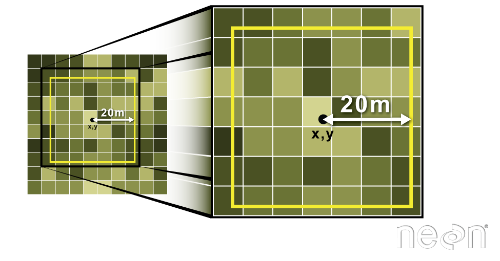
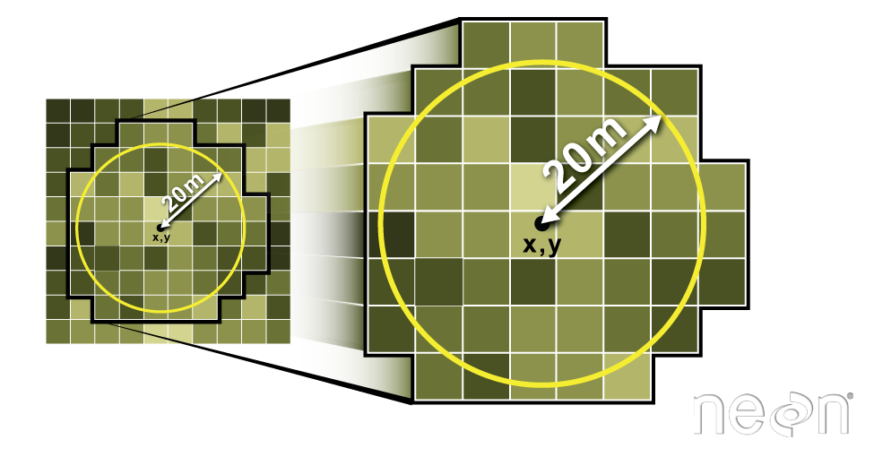
We can also extract pixel values from a raster by defining a buffer or area
surrounding individual point locations using the extract() function. To do this
we define the summary argument (fun = mean) and the buffer distance (buffer = 20)
which represents the radius of a circular region around each point. By default, the units of the
buffer are the same units as the data’s CRS. All pixels that are touched by the buffer region are included in the extract.
Source: National Ecological Observatory Network (NEON).
Let’s put this into practice by figuring out the mean tree height in the
20m around the tower location (point_HARV). Because we are extracting only a single number, we
will not use the df = TRUE argument.
mean_tree_height_tower <- extract(x = CHM_HARV,
                                  y = point_HARV,
                                  buffer = 20,
                                  fun = mean)

mean_tree_height_tower
[1] 22.38812
Challenge: Extract Raster Height Values For Plot Locations
1) Use the plot locations object (
plot_locations_sp_HARV) to extract an average tree height for the area within 20m of each vegetation plot location in the study area. Because there are multiple plot locations, there will be multiple averages returned, so thedf = TRUEargument should be used.2) Create a plot showing the mean tree height of each area.
Answers
# extract data at each plot location
mean_tree_height_plots_HARV <- extract(x = CHM_HARV,
                                       y = plot_locations_sp_HARV,
                                       buffer = 20,
                                       fun = mean,
                                       df = TRUE)

# view data
mean_tree_height_plots_HARV
ID HARV_chmCrop 1 1 NA 2 2 NA 3 3 22.35182 4 4 NA 5 5 NA 6 6 19.16891 7 7 20.61542 8 8 21.61490 9 9 NA 10 10 19.13231 11 11 21.36908 12 12 NA 13 13 17.25802 14 14 NA 15 15 12.52353 16 16 15.51574 17 17 NA 18 18 18.19454 19 19 19.67558 20 20 20.23258 21 21 NA# plot data ggplot(data = mean_tree_height_plots_HARV, aes(ID, HARV_chmCrop)) + geom_col() + ggtitle("Mean Tree Height at each Plot") + xlab("Plot ID") + ylab("Tree Height (m)")Warning: Removed 9 rows containing missing values (position_stack).

Key Points
Use the
crop()function to crop a raster object.Use the
extract()function to extract pixels from a raster object that fall within a particular extent boundary.Use the
extent()function to define an extent.