Overview

Teaching: min
Exercises: 5 min

Questions

• What are the coordinate reference systems for your rasters and are they the same?

Objectives

• Visually explore the patterns in your rasters. Reproject the your raster into UTM coordinates.

Outline

• Intro + Minute questions (10-15 min.)
• Raster Capstone (30-40 min.):
  • Load and summarize the raster data
  • Visualize the raster data
  • Develop insights
  • Reproject your raster
• Outro + Final Questions (10-15 min.)

In this capstone lesson, we use the following capstone data:

• A raster of maximum temperature in Wisconsin
• A raster of minimum temperature in Wisconsin

If you are using your own data, please identify two (2) rasters with continuous values and that are unprojected.

1) Load and summarize

Practice the first steps of using data by loading in the maximum and minimum temperature rasters for Wisconsin using the raster() function and then exploring using the summary() function.

Solution

library(raster)

Loading required package: sp

library(ggplot2)
library(rgdal)

rgdal: version: 1.5-23, (SVN revision 1121)
Geospatial Data Abstraction Library extensions to R successfully loaded
Loaded GDAL runtime: GDAL 3.0.4, released 2020/01/28
Path to GDAL shared files: /usr/share/gdal
GDAL binary built with GEOS: TRUE 
Loaded PROJ runtime: Rel. 6.3.1, February 10th, 2020, [PJ_VERSION: 631]
Path to PROJ shared files: /usr/share/proj
Linking to sp version:1.4-5
To mute warnings of possible GDAL/OSR exportToProj4() degradation,
use options("rgdal_show_exportToProj4_warnings"="none") before loading rgdal.

mintemp <- raster("../data/mintemp_monthcold_wi.tif")
summary(mintemp)

        mintemp_monthcold_wi
Min.                  -20.70
1st Qu.               -18.20
Median                -16.70
3rd Qu.               -14.45
Max.                  -11.10
NA's                  377.00

maxtemp <- raster("../data/maxtemp_monthwarm_wi.tif")
summary(maxtemp)

        maxtemp_monthwarm_wi
Min.                    24.9
1st Qu.                 26.5
Median                  27.6
3rd Qu.                 28.2
Max.                    29.0
NA's                   377.0

2) Check the CRS

Use the crs() function to check if the coordinate reference systems the same in these two rasters?

Solution

mintemp

class      : RasterLayer 
dimensions : 27, 36, 972  (nrow, ncol, ncell)
resolution : 0.1666667, 0.1666667  (x, y)
extent     : -93, -87, 42.5, 47  (xmin, xmax, ymin, ymax)
crs        : +proj=longlat +datum=WGS84 +no_defs 
source     : mintemp_monthcold_wi.tif 
names      : mintemp_monthcold_wi 
values     : -20.7, -11.1  (min, max)

maxtemp

class      : RasterLayer 
dimensions : 27, 36, 972  (nrow, ncol, ncell)
resolution : 0.1666667, 0.1666667  (x, y)
extent     : -93, -87, 42.5, 47  (xmin, xmax, ymin, ymax)
crs        : +proj=longlat +datum=WGS84 +no_defs 
source     : maxtemp_monthwarm_wi.tif 
names      : maxtemp_monthwarm_wi 
values     : 24.9, 29  (min, max)

OR

crs(mintemp)

CRS arguments: +proj=longlat +datum=WGS84 +no_defs 

crs(maxtemp)

CRS arguments: +proj=longlat +datum=WGS84 +no_defs 

Yes, the CRS for both rasters is the same. Both are in longlat projection, datum WGS84.

3) Visualize

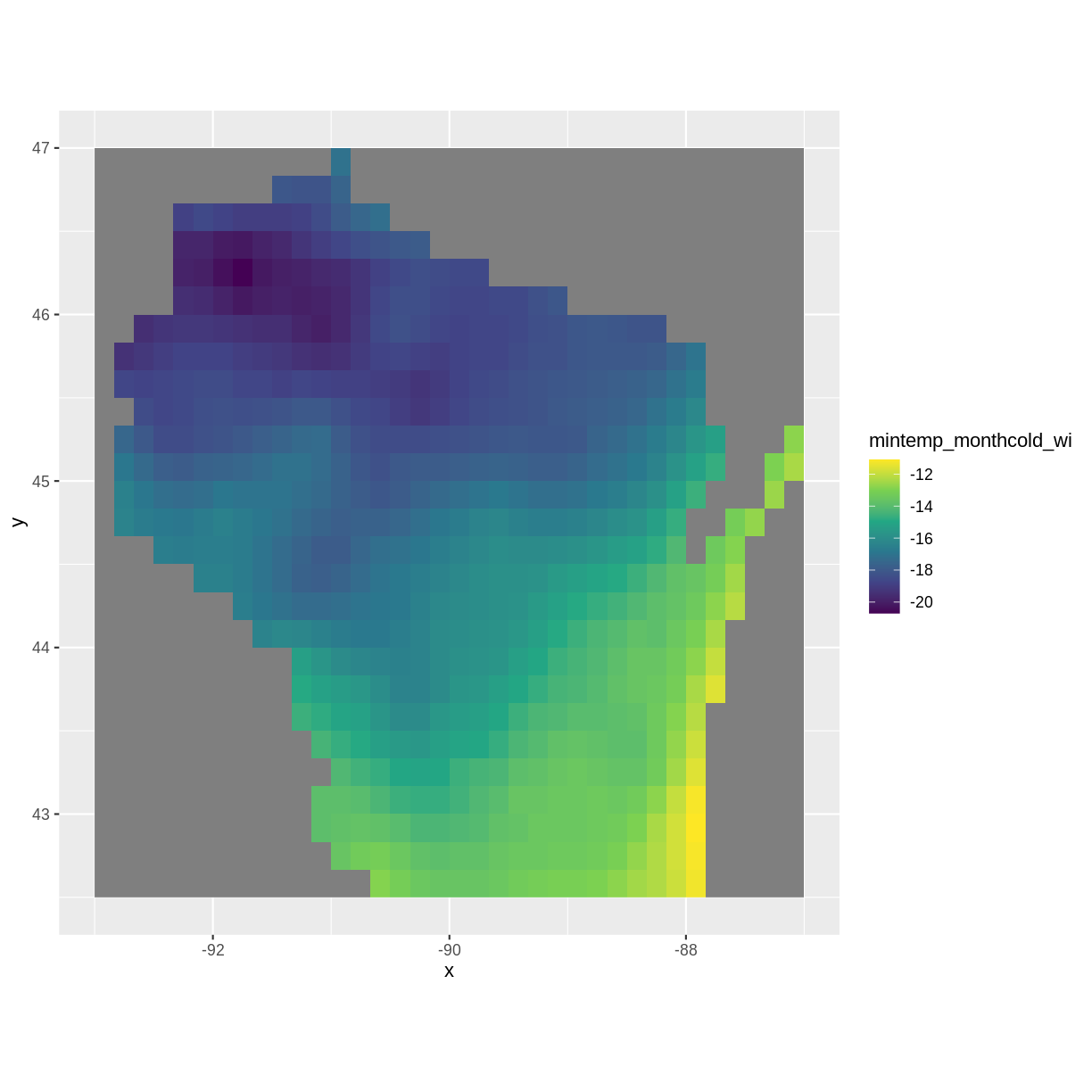
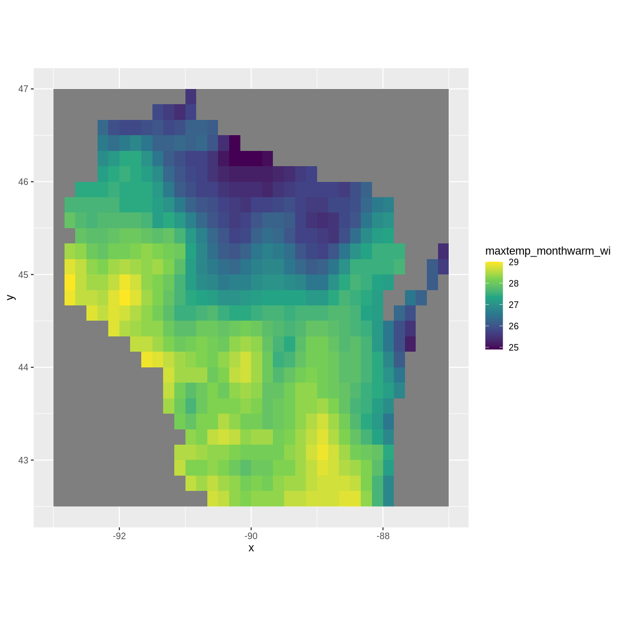
Create visualizations of both minimum and maximum temperature rasters using the ggplot2 package.

Solution

mintemp_df <- as.data.frame(mintemp, xy=TRUE)
maxtemp_df <- as.data.frame(maxtemp, xy=TRUE)

ggplot() +
   geom_raster(data = mintemp_df , aes(x = x, y = y, fill = mintemp_monthcold_wi)) +
   scale_fill_viridis_c() +
   coord_quickmap()

ggplot() +
   geom_raster(data = maxtemp_df , aes(x = x, y = y, fill = maxtemp_monthwarm_wi)) +
   scale_fill_viridis_c() +
   coord_quickmap()

Bonus

You can add the following aesthetics to a ggplot to customize the backgrounds, axis labels, title, legend label, and move the legend position to the bottom of the plot:

ggplot() +
    geom_*() +
    labs(title = "Your Title", x="X Label", y="Y Label", fill="Legend Label") +
    theme_bw() +
    theme(plot.title = element_text(hjust = 0.5), legend.position = "bottom")

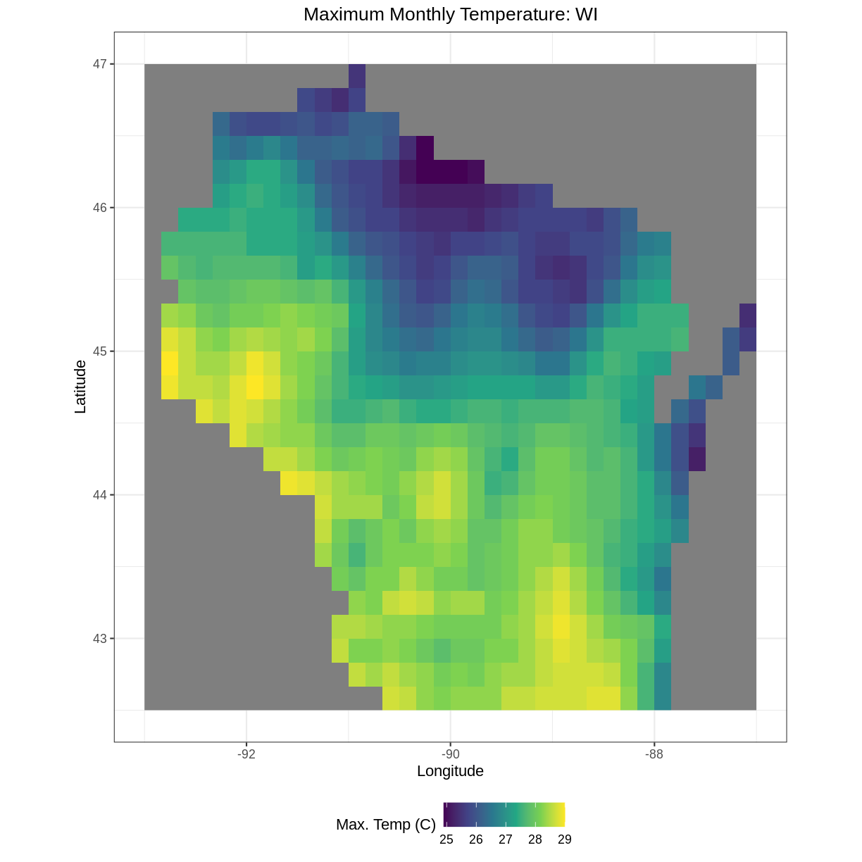
Explore what these aesthetics do with your plot of maximum monthly temperature.

Solution

ggplot() +
   geom_raster(data = maxtemp_df , aes(x = x, y = y, fill = maxtemp_monthwarm_wi)) +
   scale_fill_viridis_c() +
   coord_quickmap() +
   labs(title = "Maximum Monthly Temperature: WI", x="Longitude", y="Latitude", fill="Max. Temp (C)") +
   theme_bw() +
   theme(plot.title = element_text(hjust = 0.5), legend.position = "bottom")

4) Develop insights

Describe what patterns you observe across the state for coldest and warmest monthly temperatures in Wisconsin. What do you hypothesize is the effect of Lake Michigan?

Solution

Warmer temperatures are in Wisconsin tend toward the lower half of the state and nearer to the Minnesota border. Colder temperatures tend toward the North and near Lake Michigan, possibly due to the lake effect

5) Reproject

Reproject the maxtemp raster into UTM coordinates using the following crs string: ` +proj=utm +zone=15 +datum=WGS84 +units=m +no_defs +ellps=WGS84 +towgs84=0,0,0 `. This string was obtained from Spatial Reference Orig under PROJ4.

Solution

maxtemp_utm <- projectRaster(maxtemp, crs=" +proj=utm +zone=15 +datum=WGS84 +units=m +no_defs +ellps=WGS84 +towgs84=0,0,0 ")
crs(maxtemp_utm)

CRS arguments:
 +proj=utm +zone=15 +datum=WGS84 +units=m +no_defs 

crs(maxtemp)

CRS arguments: +proj=longlat +datum=WGS84 +no_defs 

Key Points

• Always explore your raster first using the summary() and crs() functions.

• To plot your raster with ggplot(), first convert your raster to a data frame using the as.data.frame() function and specify the argument xy=TRUE.

• You may need to reproject your raster, for which you can use the projectRaster() function.

• There are many plotting and aesthetics options in the ggplot2 package for you to explore.